Getting started with dbscan

The dbscan package provides fast implementations of density-based clustering algorithms. These algorithms can find clusters with irregular shapes and identify observations in sparse regions as noise. This vignette introduces the usual workflow with DBSCAN and briefly shows when HDBSCAN or OPTICS may be a better choice.

Installation

Install the released version from CRAN:

install.packages("dbscan")

Load the package in each R session where you want to use it:

library(dbscan)

A first clustering

We use the two-dimensional moons data included in the package. Each row is an observation and each column is a numeric feature.

data("moons")
x <- as.matrix(moons)

plot(x, pch = 19, asp = 1, main = "Moons data")

DBSCAN needs two parameters:

eps is the radius of a point’s neighborhood.
minPts is the minimum number of points, including the point itself, needed to form a dense region.

cl <- dbscan(x, eps = 0.45, minPts = 5)
cl
#> DBSCAN clustering for 100 objects.
#> Parameters: eps = 0.45, minPts = 5
#> Using euclidean distances and borderpoints = TRUE
#> The clustering contains 3 cluster(s) and 0 noise points.
#> 
#>  1  2  3 
#> 50 25 25 
#> 
#> Available fields: cluster, eps, minPts, metric, borderPoints

The cluster assignment for each observation is stored in cl$cluster. Positive integers are cluster labels and 0 denotes noise. Cluster numbers are identifiers only; their numeric order has no meaning.

table(cl$cluster)
#> 
#>  1  2  3 
#> 50 25 25
head(cl$cluster)
#> [1] 1 1 1 1 1 1

The labels can be added to the original data or used directly for plotting.

clustered <- transform(moons, cluster = factor(cl$cluster))
head(clustered)
#>             X          Y cluster
#> 1 -0.41520756  1.0357347       1
#> 2  0.05878098  0.3043343       1
#> 3  1.10937860 -0.5097378       1
#> 4  1.54094828 -0.4275496       1
#> 5  0.92909498 -0.5323878       1
#> 6 -0.86932470  0.5471548       1

plot(
  x,
  col = cl$cluster + 1L,
  pch = ifelse(cl$cluster == 0, 4, 19),
  asp = 1,
  xlab = "X",
  ylab = "Y",
  main = "DBSCAN clustering"
)

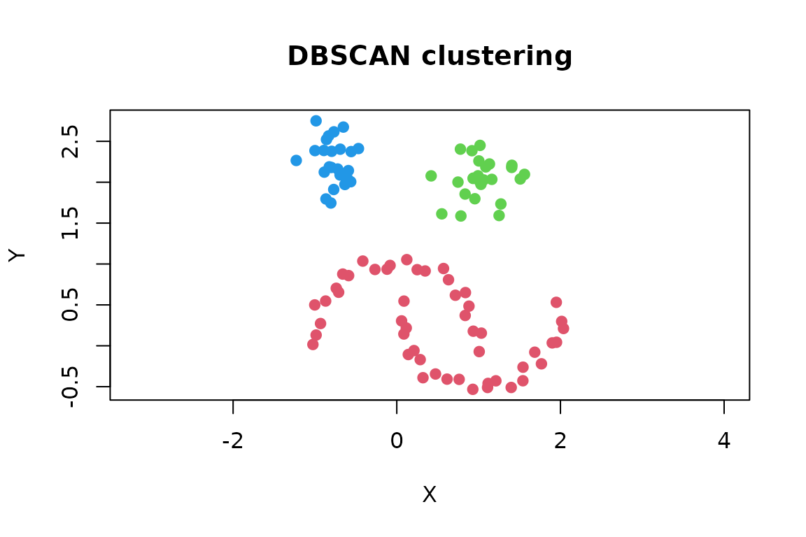
With the default R palette, noise is black because its cluster label is zero.

Prepare your own data

For the fast default search, supply a numeric matrix or data frame without missing or infinite values. DBSCAN uses Euclidean distance, so the scale of the variables matters. A variable measured in large units can otherwise dominate the distance calculation. Standardizing is often appropriate when features use different units:

x <- scale(my_data)

Whether scaling is appropriate depends on the meaning of the variables. Do not include identifiers, labels, or unordered factors as numeric features. For a non-Euclidean distance, calculate a dist object first and pass it to dbscan(); this does not use the fast kd-tree search.

Choose `minPts` and `eps`

There is no single best parameter setting for every data set. A useful starting point is:

Choose minPts based on the smallest dense group that should count as a cluster. For low-dimensional data, the number of dimensions plus one is a common lower bound; larger values produce smoother, more conservative results.
Inspect the sorted distance to each point’s minPts - 1 nearest neighbor.
Choose eps near a visible bend where the distances begin to increase rapidly.

kNNdistplot() performs the second step. Supplying minPts automatically uses k = minPts - 1 because a DBSCAN neighborhood also counts the point itself.

kNNdistplot(x, minPts = 5)
abline(h = 0.45, col = 2, lty = 2)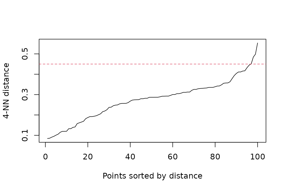

The bend is a guide rather than an automatic rule. Refit the model with a few nearby values and check whether the important structure is stable:

settings <- c(0.40, 0.45, 0.50)
fits <- lapply(
  settings,
  function(e) dbscan(x, eps = e, minPts = 5)
)

data.frame(
  eps = settings,
  clusters = vapply(fits, function(fit) max(fit$cluster), integer(1)),
  noise = vapply(fits, function(fit) sum(fit$cluster == 0), integer(1))
)
#>    eps clusters noise
#> 1 0.40        4     0
#> 2 0.45        3     0
#> 3 0.50        3     0

Increasing eps tends to merge clusters and label fewer points as noise. Increasing minPts makes the density requirement stricter. Domain knowledge and the intended use of the clusters should guide the final choice.

Assign new observations

Although DBSCAN does not learn a conventional prediction model, the package can assign a new observation to the cluster of its nearest non-noise training point within eps. If no such point exists, it is assigned to noise.

new_points <- rbind(
  c(0.0, 0.0),
  c(1.0, 2.0),
  c(4.0, 4.0)
)

predict(cl, newdata = new_points, data = x)
#> [1] 1 2 0

When training data were transformed, apply the same transformation to new observations before prediction. Also keep the original training matrix: it is required by predict().

When DBSCAN is not the best starting point

The package contains several related algorithms:

Algorithm	Useful when
`dbscan()`	Clusters have roughly similar density and one meaningful neighborhood radius can be chosen.
`hdbscan()`	Clusters may have different densities or you want to avoid choosing a global `eps`.
`optics()`	You want to explore clustering structure over a range of neighborhood radii.

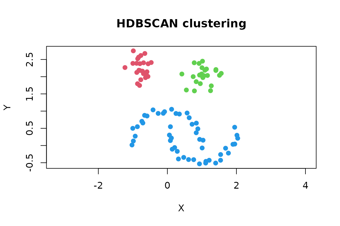
HDBSCAN requires only minPts for a basic analysis and extracts stable clusters from a density hierarchy:

hdb <- hdbscan(x, minPts = 5)
hdb
#> HDBSCAN clustering for 100 objects.
#> Parameters: minPts = 5
#> The clustering contains 3 cluster(s) and 0 noise points.
#> 
#>  1  2  3 
#> 25 25 50 
#> 
#> Available fields: cluster, minPts, coredist, cluster_scores,
#>                   membership_prob, outlier_scores, hc

plot(
  x,
  col = hdb$cluster + 1L,
  pch = ifelse(hdb$cluster == 0, 4, 19),
  asp = 1,
  main = "HDBSCAN clustering"
)

The HDBSCAN result also contains membership strengths, outlier scores, and a cluster hierarchy. See vignette("hdbscan", package = "dbscan") for a more detailed introduction.

OPTICS creates an ordering whose reachability plot exposes clustering structure. Valleys in the plot correspond to dense groups. A DBSCAN-like clustering can then be extracted at different thresholds without rerunning OPTICS.

opt <- optics(x, minPts = 5)
plot(opt)


opt_cl <- extractDBSCAN(opt, eps_cl = 0.45)
table(opt_cl$cluster)
#> 
#>  1  2  3 
#> 50 25 25

Next steps

Useful help pages include:

?dbscan for DBSCAN options, core-point detection, and more examples;
?hdbscan and ?optics for hierarchical and multi-scale clustering;
?kNN and ?frNN for fast nearest-neighbor search;
?lof and ?glosh for outlier scoring; and
?dbcv for density-based cluster validation.

For a citable description of the algorithms and implementation, use citation("dbscan").

Michael Hahsler