Nearest-Neighbor Clustering with jpclust and sNNclust

The dbscan package implements two clustering algorithms based on shared nearest neighbors:

jpclust() implements Jarvis–Patrick clustering; and
sNNclust() implements shared nearest neighbor (SNN) clustering with a DBSCAN-style density step.

Both algorithms replace the original distances between observations with a local similarity: two observations are more similar when their lists of nearest neighbors have a large overlap. This can be useful when Euclidean distance alone does not describe local cluster structure well, especially in data with irregular shapes or differing local densities.

Shared nearest neighbors

For each observation, first find its k nearest neighbors. The shared-neighbor similarity between two observations is the number of neighbors appearing in both lists. The package treats each observation as part of its own neighborhood when counting shared neighbors, and the resulting similarity is between 0 and k.

The algorithms use this information differently:

Function	Link or neighborhood rule	Cluster formation	Noise model
`jpclust()`	Mutual nearest neighbors sharing at least `kt` neighbors	Connected components	No; isolated observations form small clusters
`sNNclust()`	Mutual nearest neighbors sharing at least `eps` neighbors	DBSCAN-style core, border, and density-connected points	Yes; label `0` denotes noise

The thresholds kt and eps are counts of shared neighbors. In particular, eps in sNNclust() is not a distance radius and has a different meaning from eps in dbscan().

Example data

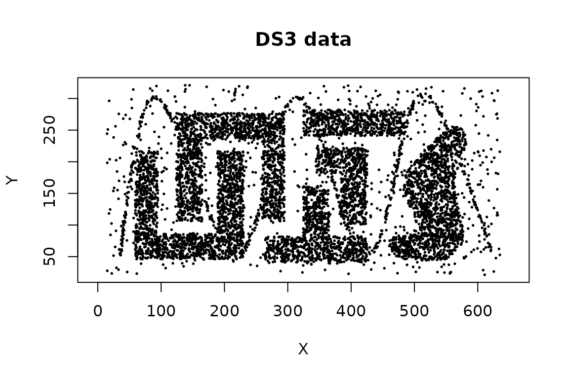
We use the DS3 data supplied with the package. It contains six irregularly-shaped groups together with noise and a sinusoidal structure that intersects the groups.

data("DS3")
x <- as.matrix(DS3)

plot(x, pch = 19, cex = 0.25, asp = 1, main = "DS3 data")

For numeric matrices and data frames, both functions use Euclidean distance and fast kd-tree nearest-neighbor search. Variable scales therefore matter. Standardize variables when their units are not comparable and scaling is appropriate for the application.

Jarvis–Patrick clustering

Jarvis–Patrick clustering links two observations when both of the following conditions hold:

Each observation is in the other’s k-nearest-neighbor list.
Their neighborhoods share at least kt neighbors.

Connected observations form clusters. Here we use neighborhoods of 20 points and require 12 shared neighbors.

jp <- jpclust(x, k = 20, kt = 12)
c(clusters = ncluster(jp), noise = nnoise(jp))
#> clusters    noise 
#>       43        0

Cluster assignments are stored in jp$cluster in the same order as the rows of x. The result also records the algorithm name, distance metric, and parameters.

names(jp)
#> [1] "cluster" "type"    "metric"  "param"
jp$param
#> $k
#> [1] 20
#> 
#> $kt
#> [1] 12
head(jp$cluster)
#> [1] 1 1 1 1 2 1

The convenience function clplot() marks observations by cluster. It uses the first two columns when the data have more than two dimensions.

clplot(x, jp, cex = 0.25, main = "Jarvis-Patrick clustering")
#> Warning in hullplot(x, cl = cl, col = col, pch = pch, cex = cex, main = main, :
#> Not enough colors. Some colors will be reused.

Jarvis–Patrick clustering has no explicit concept of noise. Observations not connected to a larger group become singleton or other small clusters rather than receiving label 0. Conversely, a chain of qualifying links can join larger structures. In this example, the sinusoidal points can connect groups that otherwise appear separate.

Increasing kt makes the link rule stricter. This removes edges from the shared-neighbor graph and can split clusters or create more small components. Decreasing kt adds edges and can merge clusters through chaining.

jp_settings <- c(10, 12, 14)
jp_fits <- lapply(
  jp_settings,
  function(threshold) jpclust(x, k = 20, kt = threshold)
)

data.frame(
  kt = jp_settings,
  clusters = vapply(jp_fits, ncluster, integer(1)),
  singleton_clusters = vapply(
    jp_fits,
    function(fit) sum(table(fit$cluster) == 1L),
    integer(1)
  )
)
#>   kt clusters singleton_clusters
#> 1 10       24                 18
#> 2 12       43                 33
#> 3 14      189                118

The required range is 1 <= kt <= k. A useful setting should preserve stable, meaningful components without fragmenting the data into many tiny clusters.

Shared nearest neighbor clustering

sNNclust() adds a density model to the shared-neighbor graph:

Build k-nearest-neighbor lists and their shared-neighbor similarities.
Retain mutual-neighbor relationships with similarity at least eps.
Treat an observation as a core point if its SNN neighborhood contains at least minPts points.
Join density-connected core points and optionally assign border points.

For the example, two neighbors must share at least 7 of their 20 neighbors, and an observation needs a sufficiently dense SNN neighborhood of at least 16 points to become a core point.

snn <- sNNclust(x, k = 20, eps = 7, minPts = 16)
snn
#> SharedNN clustering for 8000 objects.
#> Parameters: k = 20, eps = 7, minPts = 16, borderPoints = 1
#> The clustering contains 10 cluster(s) and 187 noise points.
#> 
#>    0    1    2    3    4    5    6    7    8    9   10 
#>  187 1812  740  998 1770  667 1666   76   49   20   15 
#> 
#> Available fields: cluster, type, param, metric

As with DBSCAN, positive integers are arbitrary cluster identifiers and 0 denotes noise.

clplot(x, snn, cex = 0.25, main = "Shared nearest neighbor clustering")
#> Warning in hullplot(x, cl = cl, col = col, pch = pch, cex = cex, main = main, :
#> Not enough colors. Some colors will be reused.

The parameters control different parts of the algorithm:

k determines the scale at which local neighborhoods are compared. Small values emphasize very local structure; large values smooth the similarities over a wider neighborhood.
eps is the minimum number of shared neighbors needed for an SNN relationship. Increasing it makes similarity more selective.
minPts is the density requirement in the thresholded SNN graph. Increasing it makes core-point status more difficult to attain and generally produces more noise.
borderPoints = TRUE, the default, assigns non-core observations adjacent to a core cluster. Set it to FALSE for a core-points-only result analogous to DBSCAN*.

Parameter effects interact, so inspect several nearby settings rather than selecting each value independently.

snn_settings <- data.frame(
  eps = c(5, 7, 9),
  minPts = c(16, 16, 16)
)

snn_fits <- lapply(
  seq_len(nrow(snn_settings)),
  function(i) sNNclust(
    x,
    k = 20,
    eps = snn_settings$eps[i],
    minPts = snn_settings$minPts[i]
  )
)

transform(
  snn_settings,
  clusters = vapply(snn_fits, ncluster, integer(1)),
  noise = vapply(snn_fits, nnoise, integer(1))
)
#>   eps minPts clusters noise
#> 1   5     16       10   166
#> 2   7     16       10   187
#> 3   9     16       15   213

Cluster counts alone do not identify the best solution. Examine whether the important groups persist, whether points labeled as noise are plausible, and whether conclusions are stable under small parameter changes.

Reuse a nearest-neighbor search

Nearest-neighbor search can be computed once and reused. This is especially helpful when comparing algorithms or parameter settings on a large data set. Compute at least the largest k that any later fit will need.

nn <- kNN(x, k = 30)

jp_from_nn <- jpclust(nn, k = 20, kt = 12)
snn_from_nn <- sNNclust(nn, k = 20, eps = 7, minPts = 16)

c(
  jp_same = identical(jp$cluster, jp_from_nn$cluster),
  snn_same = identical(snn$cluster, snn_from_nn$cluster)
)
#>  jp_same snn_same 
#>     TRUE     TRUE

When the full stored neighborhood should be used, k may be omitted from jpclust() because it can be recovered from the kNN object. Keep k explicit when using only the first part of a larger precomputed neighborhood.

Inspect the shared-neighbor graph

The lower-level sNN() function exposes the shared-neighbor calculation. Its shared matrix gives the similarity between each observation and each of its k nearest neighbors.

shared_nn <- sNN(nn, k = 20, jp = TRUE, sort = FALSE)
shared_nn
#> shared-nearest neighbors for 8000 objects (k=20, kt=NULL).
#> Available fields: dist, id, k, sort, metric, shared, sort_shared
table(shared_nn$shared)
#> 
#>     0     2     3     4     5     6     7     8     9    10    11    12    13 
#> 24250    20    56   204   592  1412  3094  5748  8748 11670 13902 15042 14862 
#>    14    15    16    17    18    19    20 
#> 13934 12872 11042  9236  7134  4646  1536

Using jp = TRUE reproduces the mutual-neighbor similarity used internally by sNNclust(). Use this distribution as a diagnostic when selecting a shared-neighbor threshold. sNN() can also apply a threshold directly and its graph can be inspected with adjacencylist() or plotted for small data sets; see ?sNN.

Use a precomputed distance matrix

Both clustering functions also accept a dist object. This permits other distance measures, at the cost of storing all pairwise distances and giving up the fast kd-tree search.

d <- dist(my_data, method = "manhattan")

jp_manhattan <- jpclust(d, k = 20, kt = 12)
snn_manhattan <- sNNclust(d, k = 20, eps = 7, minPts = 16)

The distance matrix must be finite. Choose a distance measure, transformations, and scaling based on the meaning of the variables rather than solely on the resulting number of clusters.

Which method should you use?

Use jpclust() when a simple connected-components interpretation of mutual shared-neighbor links is appropriate and small components are meaningful. Use sNNclust() when the analysis needs an explicit density requirement, noise labels, or control over core and border points. For either method, k sets the neighborhood scale and should reflect the smallest local structure that needs to be retained.

References

Jarvis, R. A. and Patrick, E. A. (1973). Clustering Using a Similarity Measure Based on Shared Near Neighbors. IEEE Transactions on Computers, 22(11), 1025–1034. doi:10.1109/T-C.1973.223640.

Ertoz, L., Steinbach, M., and Kumar, V. (2003). Finding Clusters of Different Sizes, Shapes, and Densities in Noisy, High Dimensional Data. Proceedings of the 2003 SIAM International Conference on Data Mining, 47–58. doi:10.1137/1.9781611972733.5.

Michael Hahsler