Using dbscan with tidyverse

The dbscan package provides tidy(), augment(), and glance() methods for its clustering algorithms, making them easy to use with tidyverse, ggplot2, and tidymodels.

Load the packages and prepare the numeric variables from the iris data:

library(dbscan)
library(tidyverse)

x <- iris[, 1:4]
db <- x %>% dbscan(eps = .42, minPts = 5)

Get cluster statistics as a tibble:

tidy(db)
#> # A tibble: 4 × 3
#>   cluster  size noise
#>   <fct>   <int> <lgl>
#> 1 0          29 TRUE 
#> 2 1          48 FALSE
#> 3 2          37 FALSE
#> 4 3          36 FALSE

The tidier augment() can be used to combine the clustering with the dataset which is useful for visualization.

augment(db, x)
#> # A tibble: 150 × 6
#>    Sepal.Length Sepal.Width Petal.Length Petal.Width .cluster noise
#>           <dbl>       <dbl>        <dbl>       <dbl> <fct>    <lgl>
#>  1          5.1         3.5          1.4         0.2 1        FALSE
#>  2          4.9         3            1.4         0.2 1        FALSE
#>  3          4.7         3.2          1.3         0.2 1        FALSE
#>  4          4.6         3.1          1.5         0.2 1        FALSE
#>  5          5           3.6          1.4         0.2 1        FALSE
#>  6          5.4         3.9          1.7         0.4 1        FALSE
#>  7          4.6         3.4          1.4         0.3 1        FALSE
#>  8          5           3.4          1.5         0.2 1        FALSE
#>  9          4.4         2.9          1.4         0.2 1        FALSE
#> 10          4.9         3.1          1.5         0.1 1        FALSE
#> # ℹ 140 more rows

Visualize the clustering with ggplot2.

augment(db, x) %>%
  ggplot(aes(x = Petal.Length, y = Petal.Width)) +
  geom_point(aes(color = .cluster, shape = noise)) +
  scale_shape_manual(values = c(19, 4))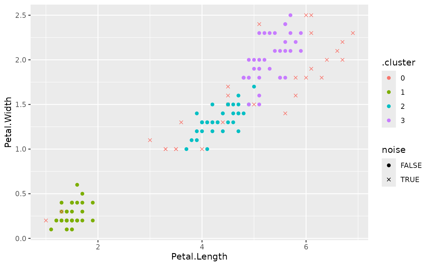

DBSCAN clusters in the iris data

scale_shape_manual() sets the point symbols to filled circles for regular points and x for noise points.

Michael Hahsler