Hierarchical DBSCAN (HDBSCAN)

Fast C++ implementation of the HDBSCAN (Hierarchical DBSCAN) and its related algorithms.

Usage

hdbscan(
  x,
  minPts,
  cluster_selection_epsilon = 0,
  gen_hdbscan_tree = FALSE,
  gen_simplified_tree = FALSE,
  verbose = FALSE
)

# S3 method for class 'hdbscan'
print(x, ...)

# S3 method for class 'hdbscan'
plot(
  x,
  scale = "suggest",
  gradient = c("yellow", "red"),
  show_flat = FALSE,
  main = "HDBSCAN*",
  ylab = "eps value",
  leaflab = "none",
  ...
)

coredist(x, minPts, ...)

mrdist(x, minPts, coredist = NULL)

# S3 method for class 'hdbscan'
predict(object, newdata, data, ...)

Arguments

x: a data matrix (Euclidean distances are used) or a dist object calculated with an arbitrary distance metric.
minPts: integer; Main parameter to control density estimate smoothing and the minimum clusters size. See details. For mrdist() (and mst_mrdist()) it can be omitted if coredist is specified.
cluster_selection_epsilon: double; a distance threshold below which no clusters should be selected (see Malzer & Baum 2020). The threshold is specified in mutual reachability distance (see mrdist()). The default of 0.0 means this feature is not used.
gen_hdbscan_tree: logical; should the robust single linkage tree be explicitly computed (see cluster tree in Chaudhuri et al, 2010).
gen_simplified_tree: logical; should the simplified hierarchy be explicitly computed (see Campello et al, 2013).
verbose: report progress.
...: additional arguments are passed on.
scale: integer; used to scale condensed tree based on the graphics device. Lower scale results in wider colored trees lines. The default 'suggest' sets scale to the number of clusters.
gradient: character vector; the colors to build the condensed tree coloring with.
show_flat: logical; whether to draw boxes indicating the most stable clusters.
main: Title of the plot.
ylab: the label for the y axis.
leaflab: a string specifying how leaves are labeled (see stats::plot.dendrogram()).
coredist: numeric vector with precomputed core distances (optional).
object: clustering object.
newdata: new data points for which the cluster membership should be predicted.
data: the data set used to create the clustering object.

Value

hdbscan() returns object of class hdbscan with the following components:

cluster: A integer vector with cluster assignments. Zero indicates noise points.
minPts: value of the minPts parameter.
cluster_scores: The sum of the stability scores for each salient (flat) cluster. Corresponds to cluster IDs given the in "cluster" element.
membership_prob: The probability or individual stability of a point within its clusters. Between 0 and 1.
outlier_scores: The GLOSH outlier score of each point.
coredist: The core distance of each data point (see coredist()).
hc: An hclust object of the HDBSCAN hierarchy (the single-linkage hierarchy of the minimum spanning tree of the mutual reachability distances before condensing). It also stores the used minPts value and can be used as input for extractFOSC().
hdbscan_tree: A dendrogram of the hierarchy. Only present if gen_hdbscan_tree = TRUE.
simplified_tree: A dendrogram of the simplified hierarchy. Only present if gen_simplified_tree = TRUE.

coredist() returns a vector with the core distance for each data point.

mrdist() returns a dist object containing pairwise mutual reachability distances.

Details

This fast implementation of HDBSCAN (Campello et al., 2013) computes the hierarchical cluster tree representing density estimates along with the stability-based flat cluster extraction. HDBSCAN essentially computes the hierarchy of all DBSCAN* clusterings, and then uses a stability-based extraction method to find optimal cuts in the hierarchy, thus producing a flat solution. It uses Prim's algorithm and is memory efficient by avoiding to create a complete distance matrix.

The algorithm

The algorithm uses as the main parameter minPts which is used in several of the HDBSCAN steps:

Compute mutual reachability distances from core distances. For core distances, minPts is a smoothing parameter for the density estimates; larger values for minPts give larger and smoother density estimates.
Construct a minimum spanning tree from the mutual reachability distances.
Prune the tree using stability. Here minPts controls the minimum cluster size because splits are only allowed when both branches have at least minPts points.
Extract the clusters from the pruned tree.

The individual steps are described in the following.

Core and mutual reachability distances

These can be calculated using the following two exposed functions:

coredist(): The core distance is defined for each point as the distance to the (minPts - 1)-th nearest neighbor. It produces a density estimate where larger values for minPts lead to larger and smoother estimates. The core distance is For matrix data, a fast k-d tree based on Euclidean distance is used. Additional parameters to coredist() are passed on to kNNdist(). A core distance vector is returned.
mrdist(): The mutual reachability distance is defined between two points as mrd(a, b) = max(coredist(a), coredist(b), dist(a, b)). It has the effect of increasing distances in low density areas, separating clusters better.

To use non-Euclidean distances, the call hdbscan(), coredist(), or mrdist() with a precomputed distance matrix.

Minimum spanning tree construction

mst_dist() constructs a MST from a data from the mutual reachability distance matrix. Since distance matrices are of size \(O(n^2)\) and thus can become very large, mst_mrdist() is also provides which directly constructs the MST from matrix data without creating the full distance matrix. This reduces memory complexity \(O(d n)\) and speeds up the calculation, but only works with Euclidean distances.

Tree pruning and cluster selection

The MST is pruned using stability and clusters are extracted in the unsupervised version implemented in extractFOSC(). Because one minPts value sets both the density smoothing and the minimum cluster size in HDBSCAN, using a different minimum cluster size requires an explicit call to extractFOSC() with the new minPts, e.g., extractFOSC(res, minPts = 20). This keeps the density estimates using the original minPtsand the hierarchy of res, but recomputed stability and cluster extraction using the new minPts value.

HDBSCAN* and DBSCAN*

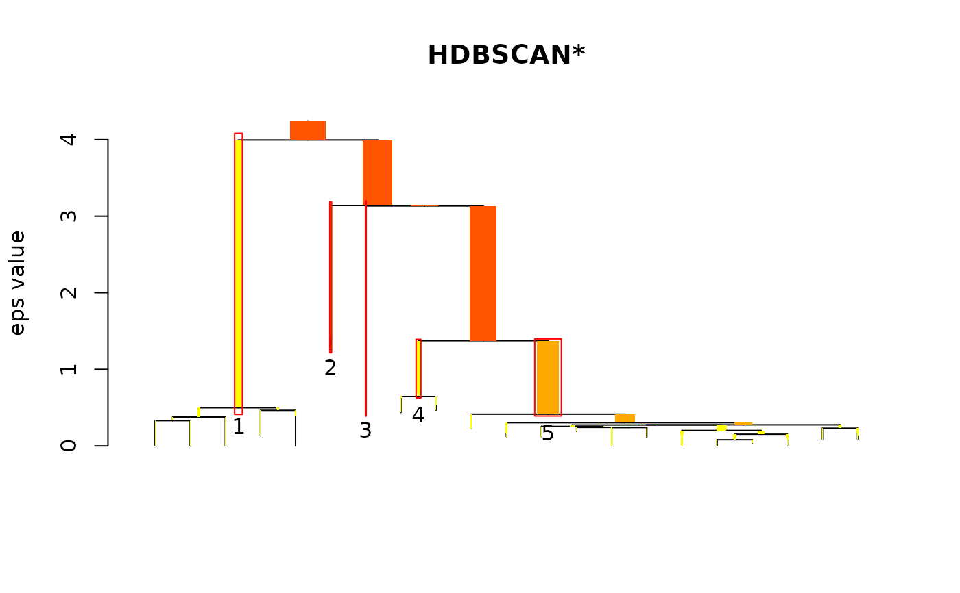
Campello, Moulavi, and Sander (2013) introduced DBSCAN* and HDBSCAN* and demonstrated that for a fixed minimum points parameter minPts, the HDBSCAN* hierarchy encodes a one-to-one correspondence with the complete set of flat clusterings obtainable by DBSCAN* across every possible radius eps. Malzer and Baum (2020) describe that a combination between DBSCAN* and HDBSCAN* can be achieved by using a cluster_selection_epsilon greater than 0.0. The tree below cluster_selection_epsilon produces a result identical to DBSCAN* with eps = cluster_selection_epsilon. The remaining part (on levels above the threshold) is still processed by HDBSCAN*'s stability-based selection algorithm and can therefore return clusters of variable densities. Note that there is not always a remaining part, especially if the parameter value is chosen too large, or if there aren't enough clusters of variable densities. In this case, the result will be equal to DBSCAN*. cluster_selection_epsilon is especially useful for cases where HDBSCAN* produces too many small clusters that need to be merged, while still being able to extract clusters of variable densities at higher levels.

Cluster membership prediction for new points

predict() assigns each new data point to the same cluster as the nearest point if it is not more than that points core distance away. Otherwise the new point is classified as a noise point (i.e., cluster ID 0).

extractFOSC() implements a more general framework for clusters selection from hierarchies (i.e., dendrograms) In addition to HDBSCAN's unsupervised cluster extraction, it also provides semisupervised methods with cluster constraints.
glosh() implements the GLOSH outlier score.

References

Campello RJGB, Moulavi D, Sander J (2013). Density-Based Clustering Based on Hierarchical Density Estimates. Proceedings of the 17th Pacific-Asia Conference on Knowledge Discovery in Databases, PAKDD 2013, Lecture Notes in Computer Science 7819, p. 160. doi:10.1007/978-3-642-37456-2_14

Campello RJGB, Moulavi D, Zimek A, Sander J (2015). Hierarchical density estimates for data clustering, visualization, and outlier detection. ACM Transactions on Knowledge Discovery from Data (TKDD), 10(5):1-51. doi:10.1145/2733381

Malzer, C., & Baum, M. (2020). A Hybrid Approach To Hierarchical Density-based Cluster Selection. In 2020 IEEE International Conference on Multisensor Fusion and Integration for Intelligent Systems (MFI), pp. 223-228. doi:10.1109/MFI49285.2020.9235263

Author

Matt Piekenbrock

Claudia Malzer (added cluster_selection_epsilon)

Examples

## cluster the moons data set with HDBSCAN
data(moons)

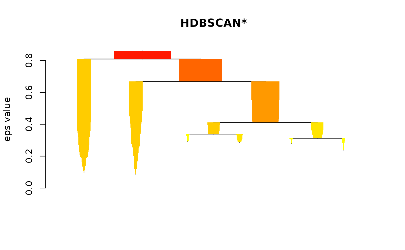
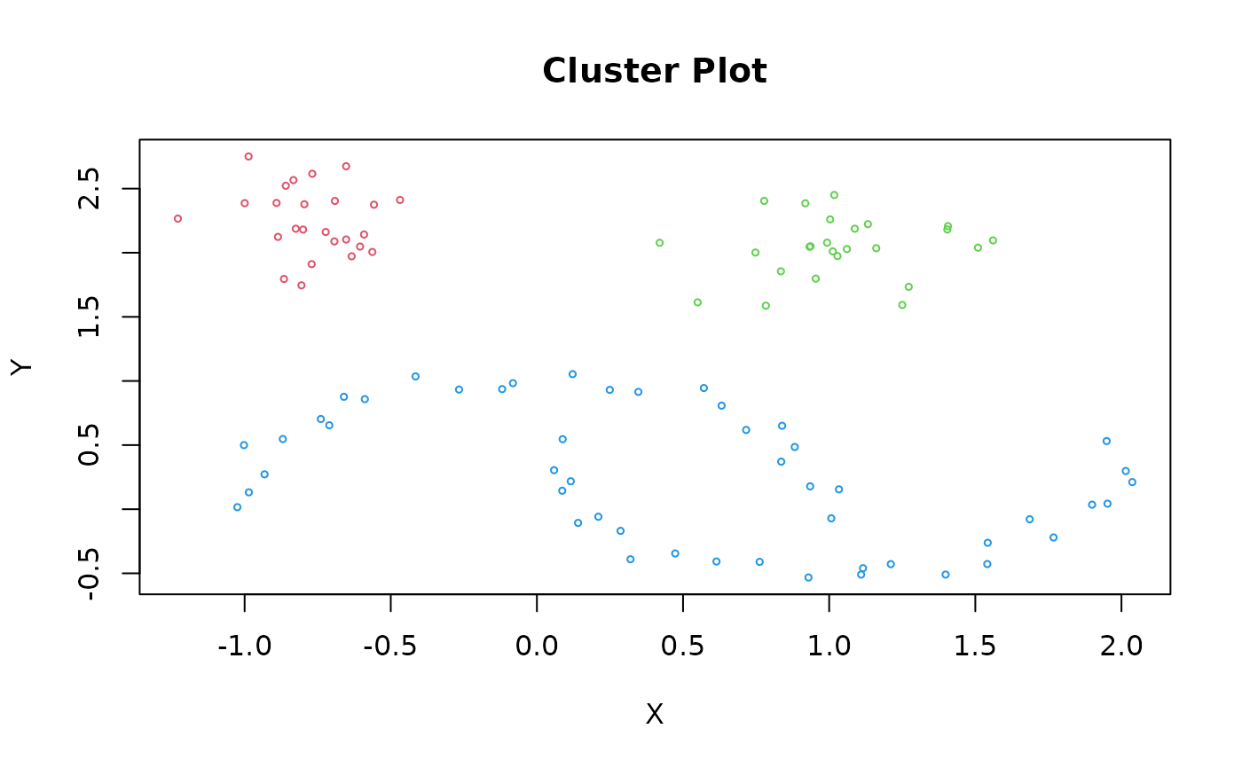
res <- hdbscan(moons, minPts = 5)
res
#> HDBSCAN clustering for 100 objects.
#> Parameters: minPts = 5
#> The clustering contains 3 cluster(s) and 0 noise points.
#> 
#>  1  2  3 
#> 25 25 50 
#> 
#> Available fields: cluster, minPts, coredist, cluster_scores,
#>                   membership_prob, outlier_scores, hc

plot(res)

clplot(moons, res)


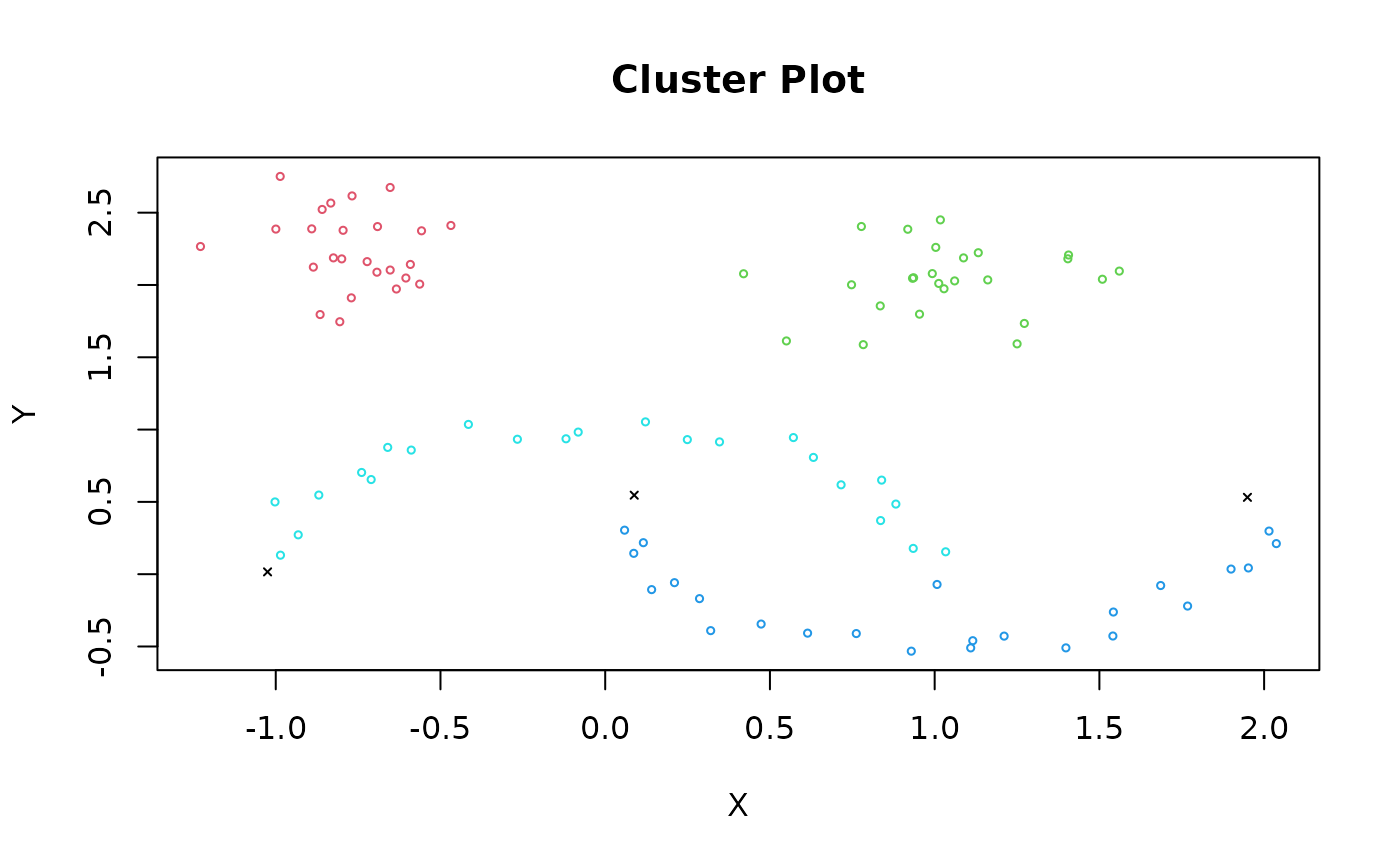
## cluster the moons data set with HDBSCAN using Manhattan distances
res <- hdbscan(dist(moons, method = "manhattan"), minPts = 5)
plot(res)

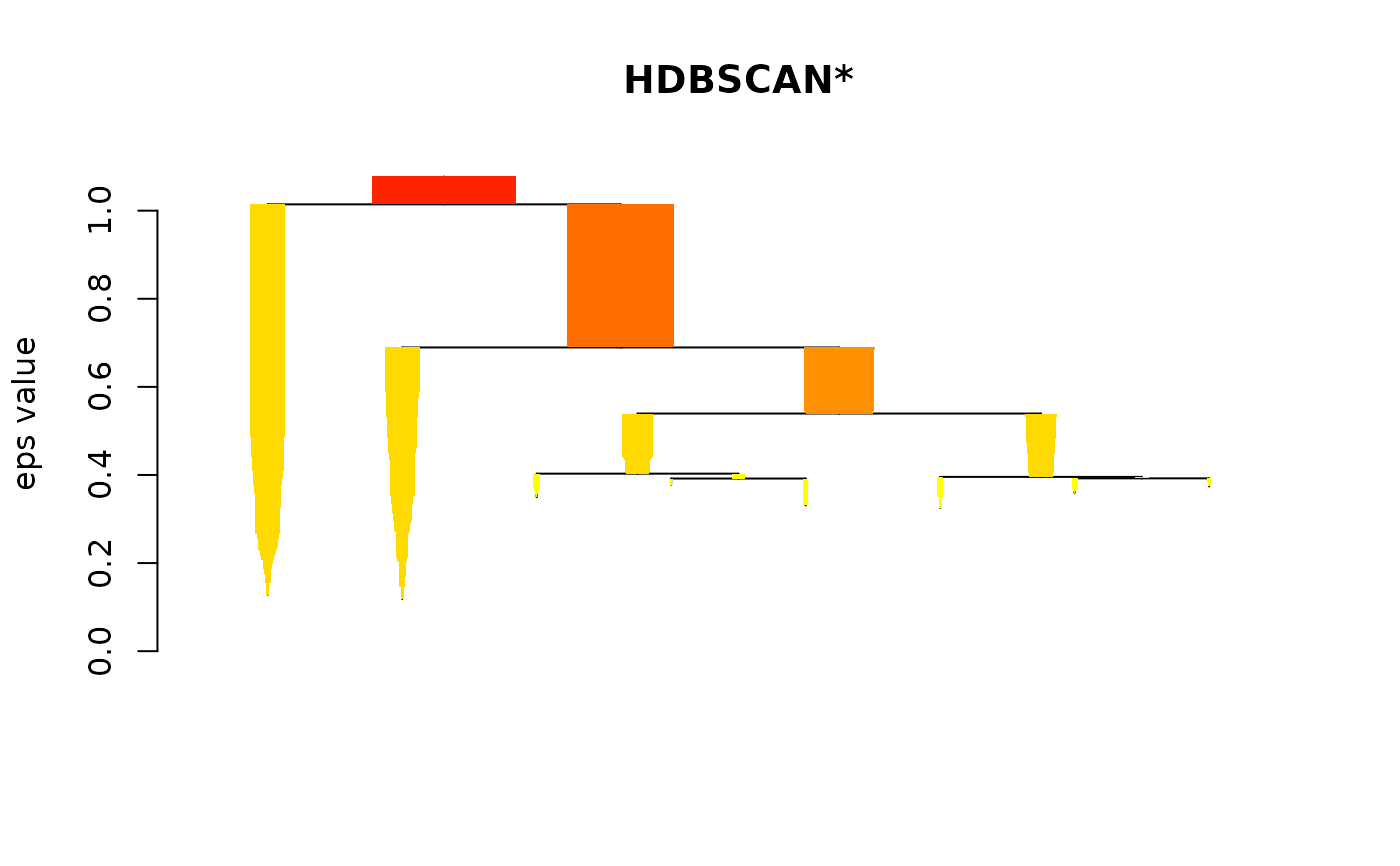clplot(moons, res)


## Example for HDBSCAN(e) using cluster_selection_epsilon
# data with clusters of various densities.
X <- data.frame(
 x = c(
  0.08, 0.46, 0.46, 2.95, 3.50, 1.49, 6.89, 6.87, 0.21, 0.15,
  0.15, 0.39, 0.80, 0.80, 0.37, 3.63, 0.35, 0.30, 0.64, 0.59, 1.20, 1.22,
  1.42, 0.95, 2.70, 6.36, 6.36, 6.36, 6.60, 0.04, 0.71, 0.57, 0.24, 0.24,
  0.04, 0.04, 1.35, 0.82, 1.04, 0.62, 0.26, 5.98, 1.67, 1.67, 0.48, 0.15,
  6.67, 6.67, 1.20, 0.21, 3.99, 0.12, 0.19, 0.15, 6.96, 0.26, 0.08, 0.30,
  1.04, 1.04, 1.04, 0.62, 0.04, 0.04, 0.04, 0.82, 0.82, 1.29, 1.35, 0.46,
  0.46, 0.04, 0.04, 5.98, 5.98, 6.87, 0.37, 6.47, 6.47, 6.47, 6.67, 0.30,
  1.49, 3.21, 3.21, 0.75, 0.75, 0.46, 0.46, 0.46, 0.46, 3.63, 0.39, 3.65,
  4.09, 4.01, 3.36, 1.43, 3.28, 5.94, 6.35, 6.87, 5.60, 5.99, 0.12, 0.00,
  0.32, 0.39, 0.00, 1.63, 1.36, 5.67, 5.60, 5.79, 1.10, 2.99, 0.39, 0.18
  ),
 y = c(
  7.41, 8.01, 8.01, 5.44, 7.11, 7.13, 1.83, 1.83, 8.22, 8.08,
  8.08, 7.20, 7.83, 7.83, 8.29, 5.99, 8.32, 8.22, 7.38, 7.69, 8.22, 7.31,
  8.25, 8.39, 6.34, 0.16, 0.16, 0.16, 1.66, 7.55, 7.90, 8.18, 8.32, 8.32,
  7.97, 7.97, 8.15, 8.43, 7.83, 8.32, 8.29, 1.03, 7.27, 7.27, 8.08, 7.27,
  0.79, 0.79, 8.22, 7.73, 6.62, 7.62, 8.39, 8.36, 1.73, 8.29, 8.04, 8.22,
  7.83, 7.83, 7.83, 8.32, 8.11, 7.69, 7.55, 7.20, 7.20, 8.01, 8.15, 7.55,
  7.55, 7.97, 7.97, 1.03, 1.03, 1.24, 7.20, 0.47, 0.47, 0.47, 0.79, 8.22,
  7.13, 6.48, 6.48, 7.10, 7.10, 8.01, 8.01, 8.01, 8.01, 5.99, 8.04, 5.22,
  5.82, 5.14, 4.81, 7.62, 5.73, 0.55, 1.31, 0.05, 0.95, 1.59, 7.99, 7.48,
  8.38, 7.12, 2.01, 1.40, 0.00, 9.69, 9.47, 9.25, 2.63, 6.89, 0.56, 3.11
 )
)

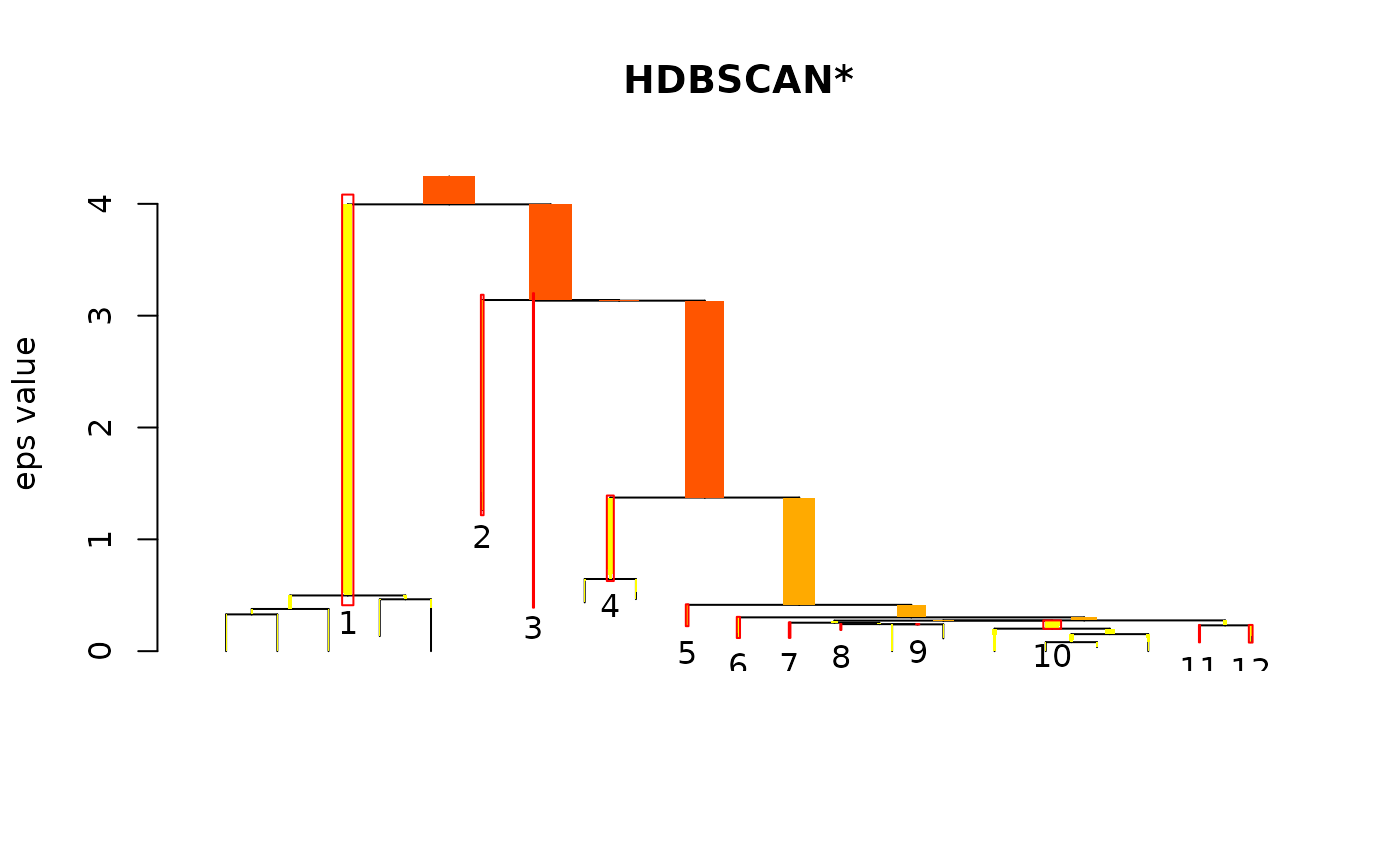
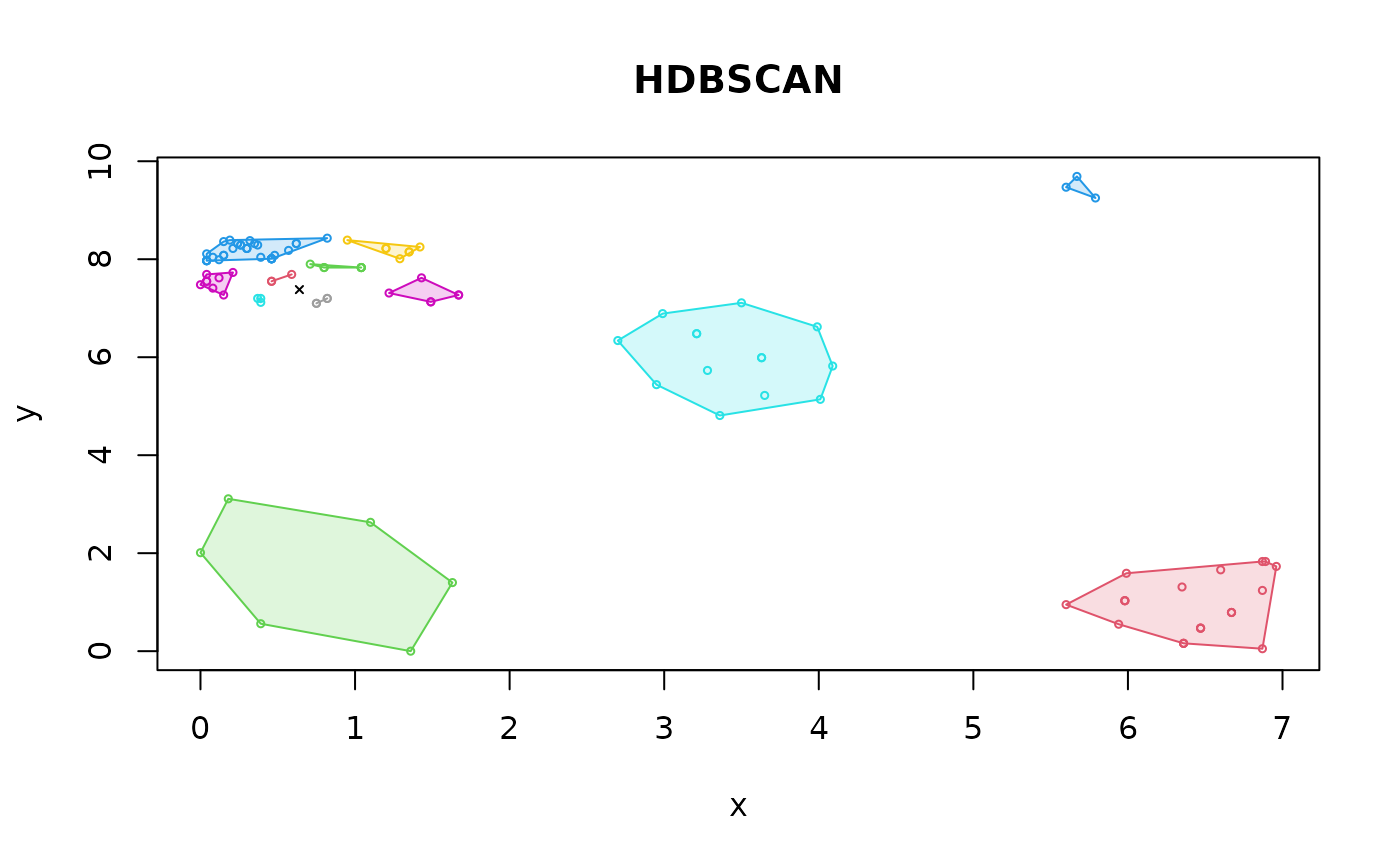
## HDBSCAN splits one cluster
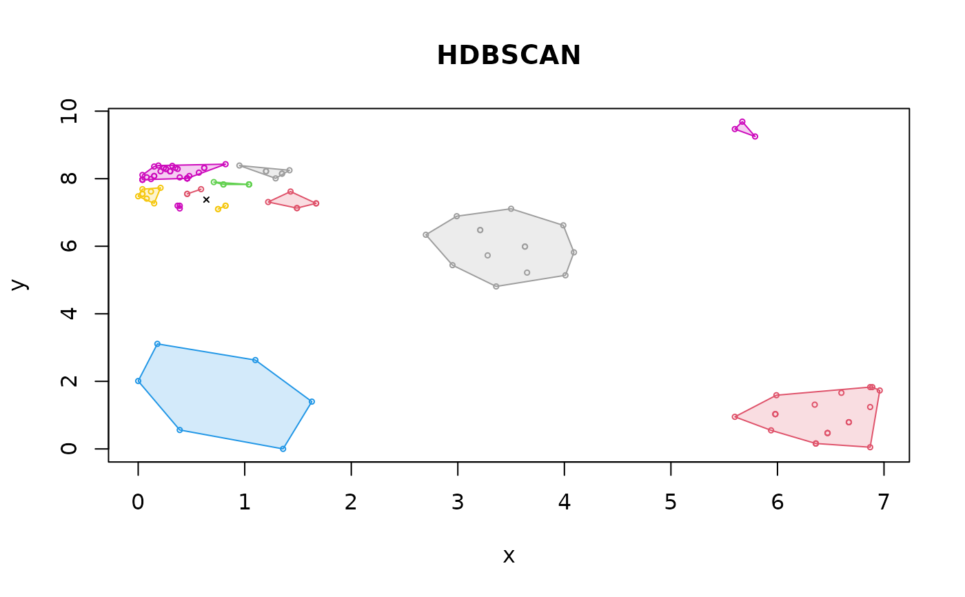
hdb <- hdbscan(X, minPts = 3)
plot(hdb, show_flat = TRUE)

hullplot(X, hdb, main = "HDBSCAN")
#> Warning: Not enough colors. Some colors will be reused.


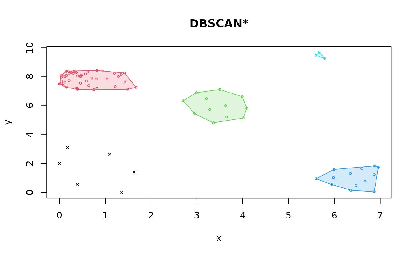
## DBSCAN* marks the least dense cluster as outliers
db <- dbscan(X, eps = 1, minPts = 3, borderPoints = FALSE)
hullplot(X, db, main = "DBSCAN*")


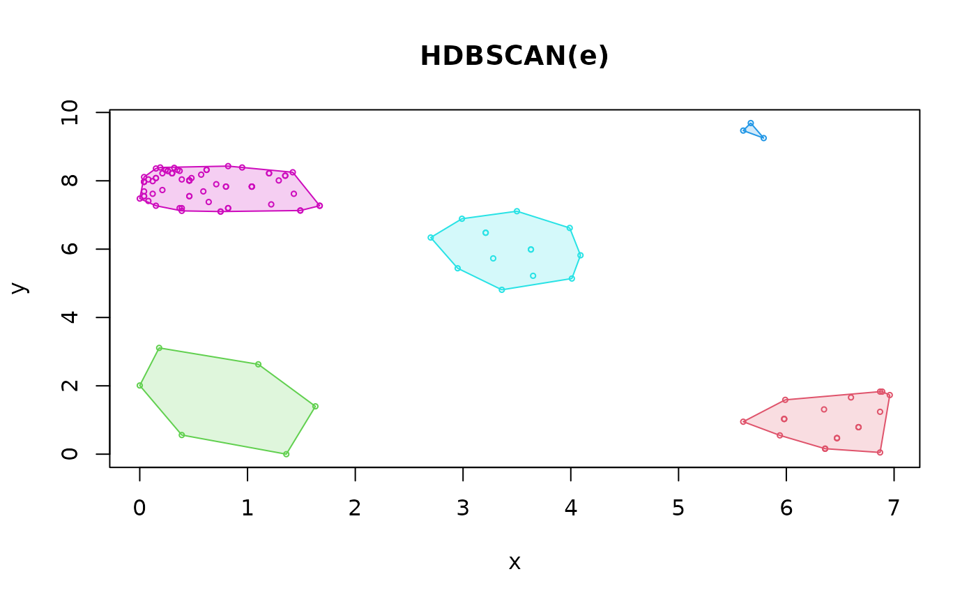
## HDBSCAN(e) mixes HDBSCAN AND DBSCAN* to find all clusters
hdbe <- hdbscan(X, minPts = 3, cluster_selection_epsilon = 1)
plot(hdbe, show_flat = TRUE)

hullplot(X, hdbe, main = "HDBSCAN(e)")


## Manually perform the steps of HDBSCAN
d <- mrdist(X, minPts = 3)
mst_hc <- mst_dist(d)
cl <- extractFOSC(mst_hc)
hullplot(X, cl$cluster, main = "HDBSCAN")
#> Warning: Not enough colors. Some colors will be reused.