Ordering Points With OPTICS

OPTICS (Ordering Points To Identify the Clustering Structure) is a density-based ordering algorithm. Like DBSCAN, it describes dense regions in terms of an epsilon neighborhood and a minimum number of points. Unlike DBSCAN, its main result is not a single clustering. OPTICS orders observations and records their reachability distances, revealing clustering structure over a range of density levels.

This vignette shows how to create and interpret an OPTICS ordering and how to extract flat or hierarchical clusters from it.

Create an OPTICS ordering

We generate four compact groups for a small reproducible example.

set.seed(2)
n <- 400
x <- cbind(
  x = runif(4, 0, 1) + rnorm(n, sd = 0.1),
  y = runif(4, 0, 1) + rnorm(n, sd = 0.1)
)

plot(x, pch = 19, asp = 1, main = "Example data")

optics() accepts a numeric matrix or data frame. For numeric data it uses Euclidean distance and a fast kd-tree search.

opt <- optics(x, minPts = 10)
opt
#> OPTICS ordering/clustering for 400 objects.
#> Parameters: minPts = 10, eps = 0.192510979570566, eps_cl = NA, xi = NA
#> Available fields: order, reachdist, coredist, predecessor, minPts, eps,
#>                   eps_cl, xi

The most important result components are:

order: row numbers of the observations in OPTICS order;
reachdist: each observation’s reachability distance; and
coredist: each observation’s core distance.

The distance vectors use the original row order. For example, reachability distances in OPTICS order are obtained with:

head(opt$order, 10)
#>  [1]   1 363 209 349 337 301 357 333 321 285
head(opt$reachdist[opt$order], 10)
#>  [1]        Inf 0.06559013 0.06559013 0.05673844 0.05673844 0.05673844
#>  [7] 0.05246930 0.05056201 0.03653219 0.03653219

The first reachability distance is undefined because the first point has no predecessor. It is stored as Inf.

Read the reachability plot

Plotting an OPTICS object produces a reachability plot. Each vertical bar is one observation, arranged in OPTICS order rather than input order.

plot(opt)

Low-reachability valleys represent dense groups. Peaks separate groups, and deeper valleys represent denser structure. The plot is therefore best read as a density landscape, not as a scatter plot or a sequence in the original data.

The ordering can also be displayed in the original coordinate space. This is mainly useful for understanding the algorithm; the reachability plot is usually clearer for real data.

plot(x, col = "grey70", pch = 19, asp = 1, main = "OPTICS order")
lines(x[opt$order, ], col = "grey40")
points(x[opt$order[1], , drop = FALSE], pch = 19, col = 2)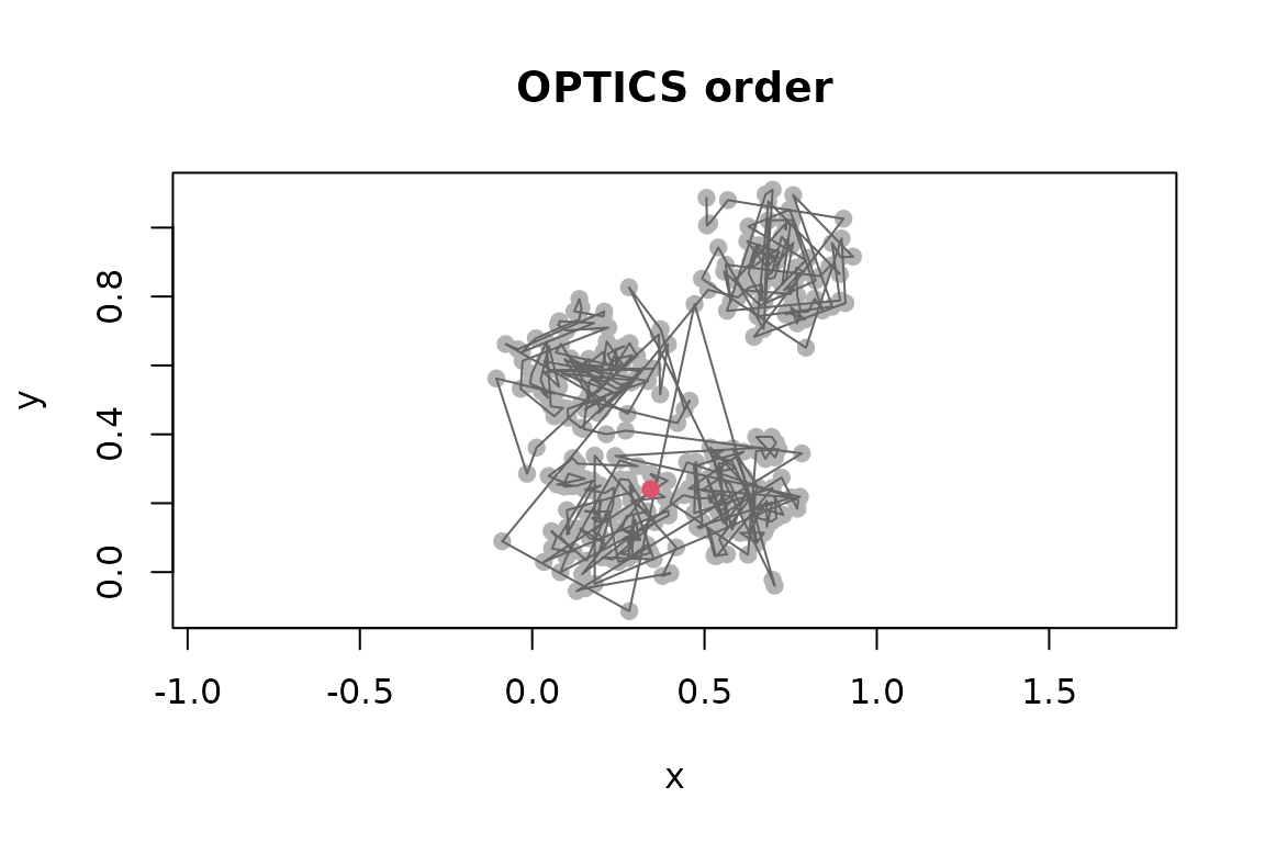

Choose `minPts` and `eps`

minPts controls the scale at which density is evaluated. It includes the point itself, so minPts = 10 uses the distance to the ninth other nearest neighbor for the core-distance calculation. Larger values average over larger neighborhoods and generally produce a smoother reachability plot; smaller values reveal finer structure but are more sensitive to local variation.

In OPTICS, eps is the maximum neighborhood radius explored by the algorithm. It is primarily a computational upper bound, not usually the density threshold used to define the final clusters. The default eps = Inf lets the package estimate a sufficient finite radius from the data and minPts.

For large data sets, supplying a smaller upper bound can reduce computation, but it must not exclude structure of interest. Multiple dashed bars in the reachability plot indicate undefined distances and usually mean that eps is too small. The first dashed bar is expected.

As with other distance-based methods, variable scales matter. Standardize variables when their units are not comparable and scaling is substantively appropriate.

Extract a DBSCAN-like clustering

extractDBSCAN() cuts the reachability plot at a global threshold eps_cl. This does not rerun OPTICS, so several thresholds can be explored using the same ordering. The extraction closely resembles DBSCAN with the same minPts and epsilon, although OPTICS can leave some DBSCAN border points unassigned.

opt_db <- extractDBSCAN(opt, eps_cl = 0.065)
opt_db
#> OPTICS ordering/clustering for 400 objects.
#> Parameters: minPts = 10, eps = 0.192510979570566, eps_cl = 0.065, xi = NA
#> The clustering contains 4 cluster(s) and 92 noise points.
#> 
#>  0  1  2  3  4 
#> 92 81 84 72 71 
#> 
#> Available fields: order, reachdist, coredist, predecessor, minPts, eps,
#>                   eps_cl, xi, cluster
plot(opt_db)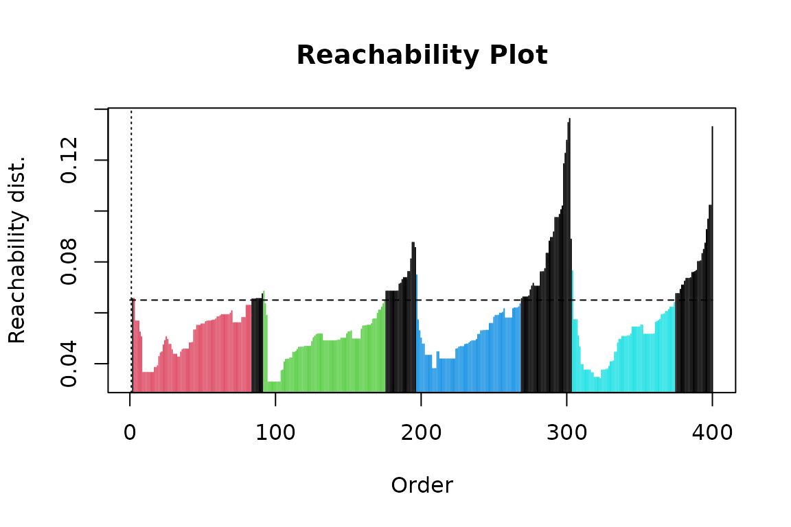

The dashed horizontal line is the extraction threshold. Bars are colored by cluster; cluster 0 is noise and appears black with the default palette. Cluster assignments are stored in original data order.

table(opt_db$cluster)
#> 
#>  0  1  2  3  4 
#> 92 81 84 72 71

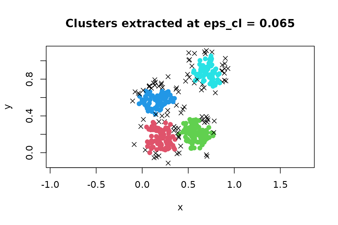
plot(
  x,
  col = opt_db$cluster + 1L,
  pch = ifelse(opt_db$cluster == 0, 4, 19),
  asp = 1,
  main = "Clusters extracted at eps_cl = 0.065"
)

Changing the cut illustrates structure at a different density level:

opt_db_wide <- extractDBSCAN(opt, eps_cl = 0.07)
c(
  clusters = max(opt_db_wide$cluster),
  noise = sum(opt_db_wide$cluster == 0)
)
#> clusters    noise 
#>        3       62

Choose eps_cl <= opt$eps. A useful threshold crosses stable valleys below the peaks that separate them. If a single global cut cannot represent groups of differing density, use the Xi extraction described next.

Extract clusters with the Xi method

extractXi() identifies relative steep-down and steep-up regions in the reachability plot. The xi value is the minimum relative change in reachability used to recognize a boundary. This can find nested clusters and clusters at different density levels without selecting one global distance threshold.

opt_xi <- extractXi(opt, xi = 0.05)
opt_xi
#> OPTICS ordering/clustering for 400 objects.
#> Parameters: minPts = 10, eps = 0.192510979570566, eps_cl = NA, xi = 0.05
#> The clustering contains 7 cluster(s) and 1 noise points.
#> 
#> Available fields: order, reachdist, coredist, predecessor, minPts, eps,
#>                   eps_cl, xi, clusters_xi, cluster
opt_xi$clusters_xi
#>   start end cluster_id
#> 1     1 194          1
#> 2     1 301          2
#> 3     8  23          3
#> 4    94 106          4
#> 5   196 288          5
#> 6   302 399          6
#> 7   308 335          7
plot(opt_xi)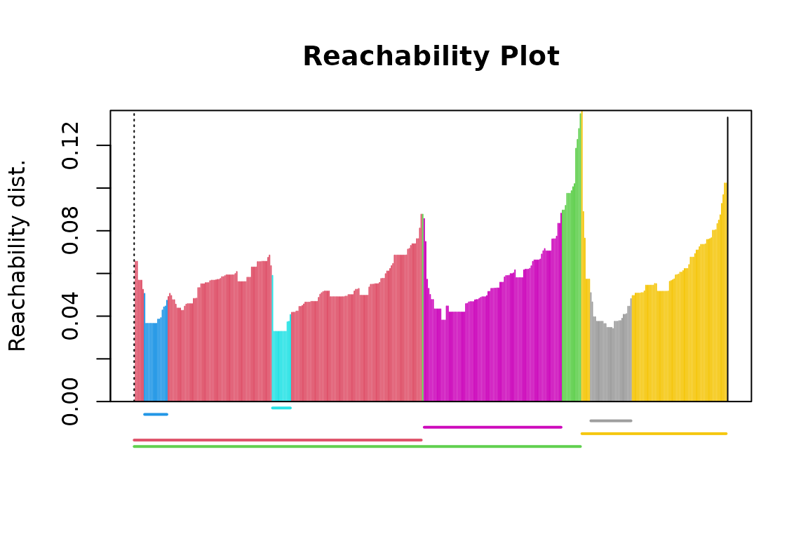

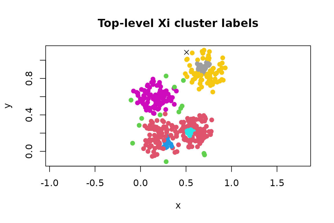
Each row of clusters_xi gives the start and end positions of a cluster in OPTICS order. These intervals can be nested. The colored line segments below the reachability plot show the intervals, while cluster contains a convenient non-nested labeling in original data order for plotting.

plot(
  x,
  col = opt_xi$cluster + 1L,
  pch = ifelse(opt_xi$cluster == 0, 4, 19),
  asp = 1,
  main = "Top-level Xi cluster labels"
)

Set minimum = TRUE to retain minimal clusters that do not contain other Xi clusters. This is useful when a non-overlapping, fine-grained solution is needed.

opt_xi_min <- extractXi(opt, xi = 0.05, minimum = TRUE)
opt_xi_min
#> OPTICS ordering/clustering for 400 objects.
#> Parameters: minPts = 10, eps = 0.192510979570566, eps_cl = NA, xi = 0.05
#> The clustering contains 4 cluster(s) and 250 noise points.
#> 
#> Available fields: order, reachdist, coredist, predecessor, minPts, eps,
#>                   eps_cl, xi, clusters_xi, cluster

The predecessor correction is enabled by default and removes a known artifact of the original Xi extraction procedure. It should normally remain enabled.

Convert the ordering to a dendrogram

An OPTICS reachability structure can be represented as a dendrogram. This is often convenient for smaller data sets or for code that works with standard R dendrogram objects.

dend <- as.dendrogram(opt)
plot(dend, leaflab = "none", ylab = "Reachability distance")

Conversion requires a complete reachability structure. If OPTICS was run with an eps that is too small, rerun it with a larger value or the default before converting.

Predict labels for new observations

Prediction is available only after extractDBSCAN(), because prediction needs a flat clustering and its global eps_cl threshold. Supply the original training data along with the new observations.

new_points <- rbind(
  c(0.2, 0.3),
  c(0.8, 0.8),
  c(2.0, 2.0)
)

predict(opt_db, newdata = new_points, data = x)
#> [1] 1 4 0

A new observation receives the label of its nearest non-noise training point within eps_cl; otherwise it is labeled 0. Apply the same transformations used for the training data to new observations.

Use another distance measure

To use a distance other than Euclidean distance, calculate a dist object and pass it to optics(). This uses the supplied pairwise distances rather than the kd-tree search.

d <- dist(x, method = "manhattan")
opt_manhattan <- optics(d, minPts = 10)
plot(opt_manhattan)

Prediction from a precomputed-distance analysis is not generally available, because distances from new observations to the training data are not stored in the dist object.

References

Ankerst, M., Breunig, M. M., Kriegel, H.-P., and Sander, J. (1999). OPTICS: Ordering Points To Identify the Clustering Structure. Proceedings of the 1999 ACM SIGMOD International Conference on Management of Data, 49–60. doi:10.1145/304181.304187.

Schubert, E. and Gertz, M. (2018). Improving the Cluster Structure Extracted from OPTICS Plots. Lernen, Wissen, Daten, Analysen (LWDA 2018), 318–329.

Hahsler, M., Piekenbrock, M., and Doran, D. (2019). dbscan: Fast Density-Based Clustering with R. Journal of Statistical Software, 91(1), 1–30. doi:10.18637/jss.v091.i01.

Michael Hahsler, Matthew Piekenbrock