
Introduction
A Markov decision process (MDP) describes sequential decision making when the state of the environment is completely observable. At every epoch, the agent observes the current state, chooses an action, receives a reward, and moves to a new state according to the transition probabilities. The objective is to find a policy that maximizes the expected sum of future rewards.
A finite-state MDP is described by states \(S\), actions \(A\), transition probabilities \(T(s' \mid s,a)\), rewards \(R(s,a,s')\), and a discount factor
\(\gamma\). The package
pomdp represents these components with an
MDP object and solves the model with
solve_MDP(). Both dynamic programming and
temporal-difference control methods are available (Sutton and Barto 2018).
The basic workflow is:
- Define a model with
MDP()or load one of the included examples. - Find a policy with
solve_MDP(). - Inspect, visualize, evaluate, or simulate the policy.
An Example MDP
We use the included Maze model. It is a gridworld with
one start state, two terminal states, and one wall. The agent can move
up, right, down, or left.
data(Maze)
Maze
#> MDP, list - Stuart Russell's 3x4 Maze
#>   Discount factor: 1
#>   Horizon: Inf epochs
#>   Size: 11 states / 4 actions
#>   Start: 0, 0, 1, 0, 0, 0, 0, 0, 0, 0, 0
#>
#>   List components: 'name', 'discount', 'horizon', 'states', 'actions',
#>     'transition_prob', 'reward', 'info', 'start'
An MDP is stored as a list. Its most important components are the states, actions, transition model, reward model, discount factor, horizon, and start distribution.
Maze$states
#>  [1] "s(1,1)" "s(2,1)" "s(3,1)" "s(1,2)" "s(3,2)" "s(1,3)" "s(2,3)" "s(3,3)"
#>  [9] "s(1,4)" "s(2,4)" "s(3,4)"
Maze$actions
#> [1] "up"    "right" "down"  "left"
Maze$discount
#> [1] 1
Maze$horizon
#> [1] Inf
Maze$start
#> s(1,1) s(2,1) s(3,1) s(1,2) s(3,2) s(1,3) s(2,3) s(3,3) s(1,4) s(2,4) s(3,4)
#>      0      0      1      0      0      0      0      0      0      0      0
Use transition_matrix() and reward_matrix()
to inspect normalized model components. For example, the following
matrix contains the transition probabilities for moving up.
transition_matrix(Maze, action = "up")
#>        s(1,1) s(2,1) s(3,1) s(1,2) s(3,2) s(1,3) s(2,3) s(3,3) s(1,4) s(2,4)
#> s(1,1)    0.9    0.0    0.0    0.1    0.0    0.0    0.0    0.0    0.0    0.0
#> s(2,1)    0.8    0.2    0.0    0.0    0.0    0.0    0.0    0.0    0.0    0.0
#> s(3,1)    0.0    0.8    0.1    0.0    0.1    0.0    0.0    0.0    0.0    0.0
#> s(1,2)    0.1    0.0    0.0    0.8    0.0    0.1    0.0    0.0    0.0    0.0
#> s(3,2)    0.0    0.0    0.1    0.0    0.8    0.0    0.0    0.1    0.0    0.0
#> s(1,3)    0.0    0.0    0.0    0.1    0.0    0.8    0.0    0.0    0.1    0.0
#> s(2,3)    0.0    0.0    0.0    0.0    0.0    0.8    0.1    0.0    0.0    0.1
#> s(3,3)    0.0    0.0    0.0    0.0    0.1    0.0    0.8    0.0    0.0    0.0
#> s(1,4)    0.0    0.0    0.0    0.0    0.0    0.0    0.0    0.0    1.0    0.0
#> s(2,4)    0.0    0.0    0.0    0.0    0.0    0.0    0.0    0.0    0.0    1.0
#> s(3,4)    0.0    0.0    0.0    0.0    0.0    0.0    0.0    0.1    0.0    0.8
#>        s(3,4)
#> s(1,1)    0.0
#> s(2,1)    0.0
#> s(3,1)    0.0
#> s(1,2)    0.0
#> s(3,2)    0.0
#> s(1,3)    0.0
#> s(2,3)    0.0
#> s(3,3)    0.1
#> s(1,4)    0.0
#> s(2,4)    0.0
#> s(3,4)    0.1
Models can be created directly with MDP(). Transition
probabilities can be specified as matrices, data frames built with
T_(), or functions. Rewards can similarly be specified as
matrices, data frames built with R_(), or functions. See
?MDP for complete examples and the supported shortcuts.
Solving an Infinite-Horizon MDP
solve_MDP() provides two model-based dynamic programming
methods and three model-free temporal-difference methods:
-
"value_iteration"applies Bellman optimality backups until the value function converges. -
"policy_iteration"alternates approximate policy evaluation and greedy policy improvement. -
"q_learning"learns an off-policy action-value function. -
"sarsa"learns an action-value function on-policy. -
"expected_sarsa"uses the expected value under the current policy in its update.
Value iteration is the default. It is a good starting point when the complete transition and reward models are available.
maze_solved <- solve_MDP(Maze, method = "value_iteration")
maze_solved
#> MDP, list - Stuart Russell's 3x4 Maze
#>   Discount factor: 1
#>   Horizon: Inf epochs
#>   Size: 11 states / 4 actions
#>   Start: 0, 0, 1, 0, 0, 0, 0, 0, 0, 0, 0
#>   Solved:
#>     Method: 'value iteration'
#>     Solution converged: TRUE
#>
#>   List components: 'name', 'discount', 'horizon', 'states', 'actions',
#>     'transition_prob', 'reward', 'info', 'start', 'solution'
The returned object contains the original model and a
solution component. For an infinite-horizon dynamic
programming solution, the latter records the method, convergence status,
final value-function change, number of iterations, and policy.
maze_solved$solution[c("method", "converged", "delta", "iterations")]
#> $method
#> [1] "value iteration"
#>
#> $converged
#> [1] TRUE
#>
#> $delta
#> [1] 0.009858138
#>
#> $iterations
#> [1] 13
policy() extracts the solution as one row per state. The
column U is the expected discounted return from that state,
and action is the action selected by the policy.
policy(maze_solved)
#>     state         U action
#> 1  s(1,1) 0.8513071  right
#> 2  s(2,1) 0.8007595     up
#> 3  s(3,1) 0.7409561     up
#> 4  s(1,2) 0.9077989  right
#> 5  s(3,2) 0.6842791   left
#> 6  s(1,3) 0.9578061  right
#> 7  s(2,3) 0.7002680     up
#> 8  s(3,3) 0.6321148   left
#> 9  s(1,4) 0.0000000   down
#> 10 s(2,4) 0.0000000   left
#> 11 s(3,4) 0.4045407   left
The action-value function \(Q(s,a)\) gives the expected return from taking action \(a\) in state \(s\) and then following the policy. It is useful for comparing the available actions in each state.
round(q_values_MDP(maze_solved), 2)
#>           up right down left
#> s(1,1)  0.82  0.85 0.78 0.81
#> s(2,1)  0.80  0.76 0.71 0.76
#> s(3,1)  0.74  0.66 0.70 0.71
#> s(1,2)  0.87  0.91 0.87 0.82
#> s(3,2)  0.64  0.60 0.64 0.69
#> s(1,3)  0.92  0.96 0.71 0.85
#> s(2,3)  0.70 -0.65 0.44 0.68
#> s(3,3)  0.63  0.42 0.57 0.64
#> s(1,4)  0.00  0.00 0.00 0.00
#> s(2,4)  0.00  0.00 0.00 0.00
#> s(3,4) -0.70  0.23 0.39 0.41
The value function and the gridworld policy can also be visualized.
plot_value_function(maze_solved)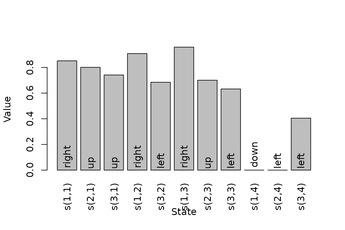
gridworld_plot_policy(maze_solved)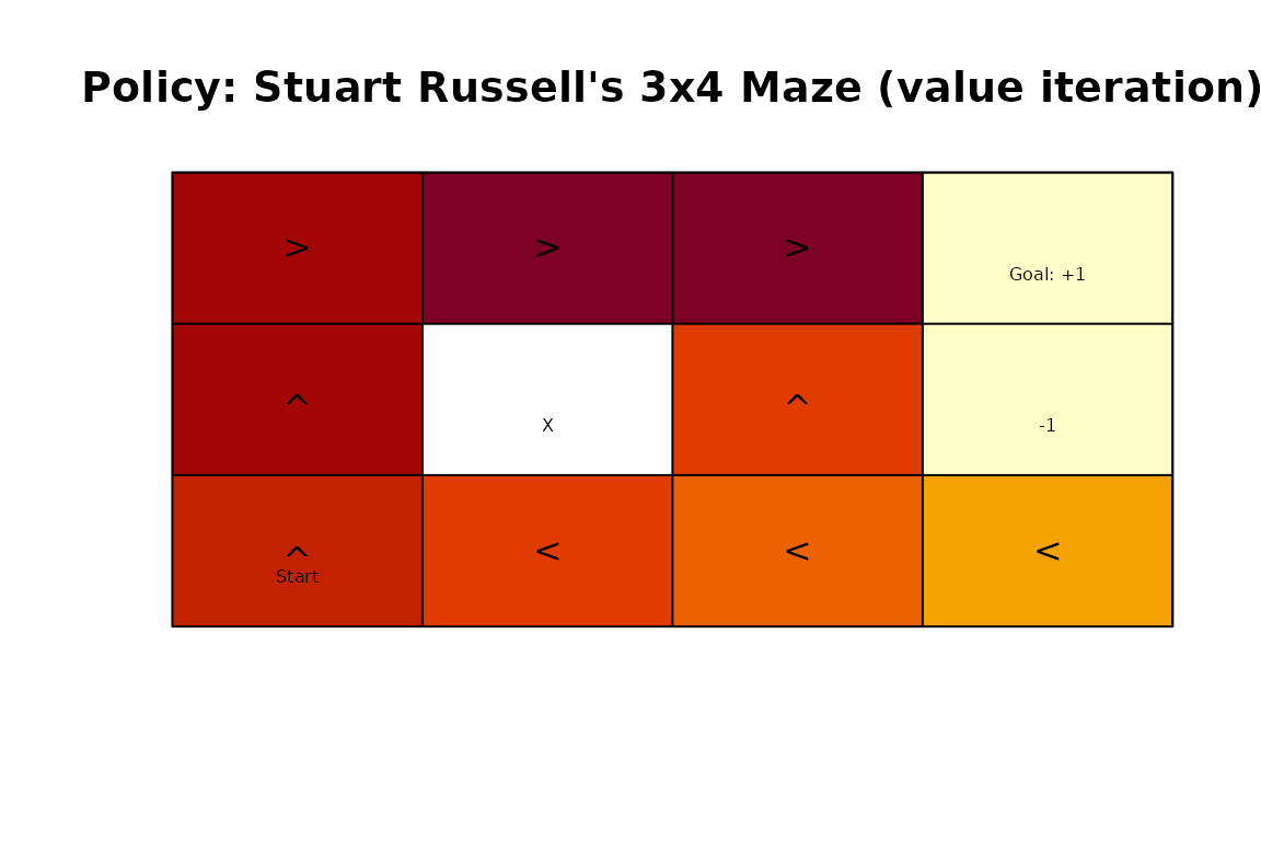
Choosing Dynamic Programming Parameters
For value iteration, error controls the maximum policy
loss used in the convergence criterion, while N_max limits
the number of iterations. An initial value function can be supplied with
U.
maze_precise <- solve_MDP(
  Maze,
  method = "value_iteration",
  error = 1e-5,
  N_max = 1000
)
maze_precise$solution[c("converged", "delta", "iterations")]
#> $converged
#> [1] TRUE
#>
#> $delta
#> [1] 9.760517e-06
#>
#> $iterations
#> [1] 25
Modified policy iteration starts with a random policy. In each
iteration it uses k_backups Bellman backups to
approximately evaluate the current policy, then replaces it with a
greedy policy. It stops when the policy no longer changes.
maze_policy_iteration <- solve_MDP(
  Maze,
  method = "policy_iteration",
  k_backups = 10
)
maze_policy_iteration$solution[c("converged", "iterations")]
#> $converged
#> [1] TRUE
#>
#> $iterations
#> [1] 5
policy(maze_policy_iteration)
#>     state         U action
#> 1  s(1,1) 0.8515581  right
#> 2  s(2,1) 0.8015579     up
#> 3  s(3,1) 0.7453018     up
#> 4  s(1,2) 0.9078082  right
#> 5  s(3,2) 0.6952879   left
#> 6  s(1,3) 0.9578082  right
#> 7  s(2,3) 0.7002740     up
#> 8  s(3,3) 0.6513679   left
#> 9  s(1,4) 0.0000000   down
#> 10 s(2,4) 0.0000000     up
#> 11 s(3,4) 0.4277575   left
The two dynamic programming methods may make different choices when actions have the same value, but their policies have the same optimal value function.
Finite-Horizon Problems
For a finite horizon, the best action can depend on how many epochs
remain. Specify the number of epochs with horizon.
Finite-horizon solving currently uses value iteration and returns one
policy per epoch.
maze_finite <- solve_MDP(
  Maze,
  method = "value_iteration",
  horizon = 3
)
policy(maze_finite)
#> [[1]]
#>     state        U action
#> 1  s(1,1)  0.41248  right
#> 2  s(2,1) -0.12000     up
#> 3  s(3,1) -0.12000  right
#> 4  s(1,2)  0.77088  right
#> 5  s(3,2) -0.12000   down
#> 6  s(1,3)  0.92808  right
#> 7  s(2,3)  0.60712     up
#> 8  s(3,3)  0.33888     up
#> 9  s(1,4)  0.00000   left
#> 10 s(2,4)  0.00000   down
#> 11 s(3,4) -0.12000   down
#>
#> [[2]]
#>     state       U action
#> 1  s(1,1) -0.0800  right
#> 2  s(2,1) -0.0800  right
#> 3  s(3,1) -0.0800     up
#> 4  s(1,2)  0.5856  right
#> 5  s(3,2) -0.0800     up
#> 6  s(1,3)  0.8672  right
#> 7  s(2,3)  0.4936     up
#> 8  s(3,3) -0.0800     up
#> 9  s(1,4)  0.0000     up
#> 10 s(2,4)  0.0000   down
#> 11 s(3,4) -0.0800   down
#>
#> [[3]]
#>     state      U action
#> 1  s(1,1) -0.040  right
#> 2  s(2,1) -0.040   left
#> 3  s(3,1) -0.040  right
#> 4  s(1,2) -0.040   left
#> 5  s(3,2) -0.040     up
#> 6  s(1,3)  0.792  right
#> 7  s(2,3) -0.040   left
#> 8  s(3,3) -0.040   down
#> 9  s(1,4)  0.000     up
#> 10 s(2,4)  0.000   down
#> 11 s(3,4) -0.040   down
Individual epochs can be extracted or plotted separately.
finite_policy <- policy(maze_finite, drop = FALSE)
finite_policy[[1]]
#>     state        U action
#> 1  s(1,1)  0.41248  right
#> 2  s(2,1) -0.12000     up
#> 3  s(3,1) -0.12000  right
#> 4  s(1,2)  0.77088  right
#> 5  s(3,2) -0.12000   down
#> 6  s(1,3)  0.92808  right
#> 7  s(2,3)  0.60712     up
#> 8  s(3,3)  0.33888     up
#> 9  s(1,4)  0.00000   left
#> 10 s(2,4)  0.00000   down
#> 11 s(3,4) -0.12000   down
finite_policy[[3]]
#>     state      U action
#> 1  s(1,1) -0.040  right
#> 2  s(2,1) -0.040   left
#> 3  s(3,1) -0.040  right
#> 4  s(1,2) -0.040   left
#> 5  s(3,2) -0.040     up
#> 6  s(1,3)  0.792  right
#> 7  s(2,3) -0.040   left
#> 8  s(3,3) -0.040   down
#> 9  s(1,4)  0.000     up
#> 10 s(2,4)  0.000   down
#> 11 s(3,4) -0.040   down
gridworld_plot_policy(maze_finite, epoch = 1)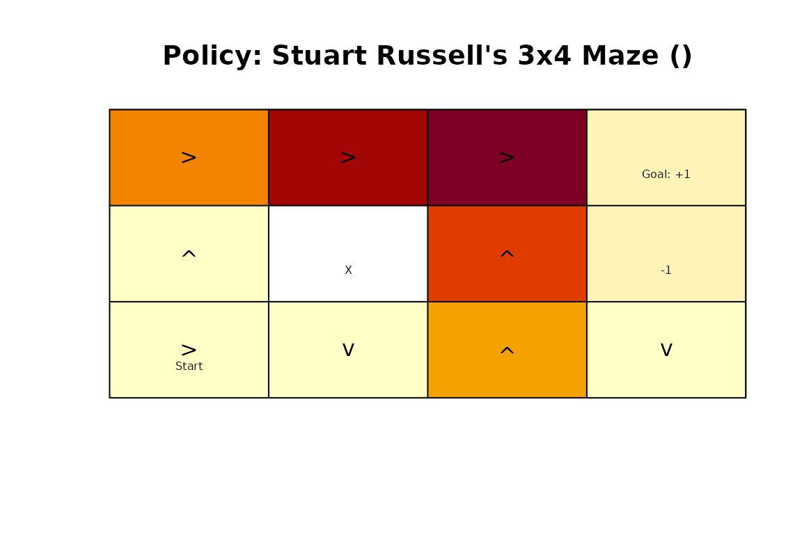
Learning from Simulated Experience
The temporal-difference methods use the MDP model only to simulate
interaction with the environment. They are useful for experimenting with
reinforcement learning. Their main controls are the number of episodes
N, learning rate alpha, exploration rate
epsilon, and maximum episode length horizon.
Models with no absorbing state require a finite
horizon.
The algorithms involve random exploration, so set a seed when reproducibility is important.
set.seed(1234)
maze_q_learning <- solve_MDP(
  Maze,
  method = "q_learning",
  N = 1000,
  alpha = 0.1,
  epsilon = 0.1
)
policy(maze_q_learning)
#>     state         U action
#> 1  s(1,1) 0.8239701  right
#> 2  s(2,1) 0.7631532     up
#> 3  s(3,1) 0.6981705     up
#> 4  s(1,2) 0.8905822  right
#> 5  s(3,2) 0.4097767   left
#> 6  s(1,3) 0.9574402  right
#> 7  s(2,3) 0.6356223     up
#> 8  s(3,3) 0.3487937     up
#> 9  s(1,4) 0.0000000   down
#> 10 s(2,4) 0.0000000   down
#> 11 s(3,4) 0.2970429   left
Q-learning is off-policy: it explores with an epsilon-greedy behavior policy while learning a greedy target policy. Sarsa and expected Sarsa instead learn from the current behavior policy. Because these methods estimate a solution from sampled experience, their learned values and policies can vary between runs and generally require parameter tuning.
Evaluating and Simulating a Policy
MDP_policy_evaluation() applies Bellman backups to
estimate the value of a given policy. This is useful for comparing an
optimal policy with a manually specified or random policy.
set.seed(1234)
random_policy <- random_MDP_policy(Maze)

rbind(
  random = MDP_policy_evaluation(random_policy, Maze),
  optimal = MDP_policy_evaluation(policy(maze_solved), Maze)
)
#>             s(1,1)     s(2,1)     s(3,1)     s(1,2)    s(3,2)     s(1,3)
#> random  -4.1644261 -3.7740116 -2.9911696 -3.0378368 -2.843810 -2.9882765
#> optimal  0.8515562  0.8015515  0.7452441  0.9078082  0.695123  0.9578082
#>            s(2,3)     s(3,3) s(1,4) s(2,4)     s(3,4)
#> random  -2.195218 -2.2998637      0      0 -2.1952182
#> optimal  0.700274  0.6510268      0      0  0.4271197
simulate_MDP() follows a solved policy through the
environment. It reports the average discounted reward and visitation
counts, and can optionally return complete trajectories.
set.seed(1234)
simulation <- simulate_MDP(
  maze_solved,
  n = 1000,
  horizon = 20,
  return_trajectories = TRUE
)
simulation$avg_reward
#> [1] 0.761
head(simulation$trajectories)
#>   episode time      s     a     r s_prime
#> 1       1    0 s(3,1)    up -0.04  s(2,1)
#> 2       1    1 s(2,1)    up -0.04  s(1,1)
#> 3       1    2 s(1,1) right -0.04  s(1,2)
#> 4       1    3 s(1,2) right -0.04  s(1,2)
#> 5       1    4 s(1,2) right -0.04  s(1,3)
#> 6       1    5 s(1,3) right  1.00  s(1,4)
Simulation is especially helpful for checking how a policy behaves from a particular start distribution, estimating its realized reward, and diagnosing states or actions that occur frequently.
Next Steps
The Maze, Cliff_walking,
Windy_gridworld, and DynaMaze data sets
provide additional MDP examples. See
vignette("gridworlds", package = "pomdp") for tools that
build and visualize gridworld MDPs, and ?solve_MDP for all
solver parameters.