Extract the Policy from a POMDP/MDP

Extracts the policy from a solved POMDP/MDP.

Usage

policy(x, drop = TRUE)

Arguments

x: A solved POMDP or MDP object.
drop: logical; drop the list for converged, epoch-independent policies.

Value

A list with the policy for each epoch. Converged policies have only one element. If drop = TRUE then the policy is returned without a list.

Details

A list (one entry per epoch) with the optimal policy. For converged, infinite-horizon problems solutions, a list with only the converged solution is produced. For a POMDP, the policy is a data.frame consisting of:

Part 1: The alpha vectors for the belief states (defines also the utility of the belief). The columns have the names of states.
Part 2: The last column named action contains the prescribed action.

For an MDP, the policy is a data.frame with columns for:

state: The state.
U: The state's value (discounted expected utility U) if the policy is followed
action: The prescribed action.

Author

Michael Hahsler

Examples

data("Tiger")

# Infinite horizon
sol <- solve_POMDP(model = Tiger)
sol
#> POMDP, list - Tiger Problem
#>   Discount factor: 0.75
#>   Horizon: Inf epochs
#>   Size: 2 states / 3 actions / 2 obs.
#>   Start: uniform
#>   Solved:
#>     Method: ‘grid’
#>     Solution converged: TRUE
#>     # of alpha vectors: 5
#>     Total expected reward: 1.933439
#> 
#>   List components: ‘name’, ‘discount’, ‘horizon’, ‘states’, ‘actions’,
#>     ‘observations’, ‘transition_prob’, ‘observation_prob’, ‘reward’,
#>     ‘start’, ‘info’, ‘solution’

# policy with value function, optimal action and transitions for observations.
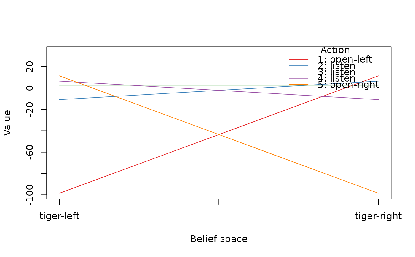
policy(sol)
#>   tiger-left tiger-right     action
#> 1 -98.549921   11.450079  open-left
#> 2 -10.854299    6.516937     listen
#> 3   1.933439    1.933439     listen
#> 4   6.516937  -10.854299     listen
#> 5  11.450079  -98.549921 open-right
plot_value_function(sol)


# Finite horizon (we use incremental pruning because grid does not converge)
sol <- solve_POMDP(model = Tiger, method = "incprune", 
  horizon = 3, discount = 1)
sol
#> POMDP, list - Tiger Problem
#>   Discount factor: 1
#>   Horizon: 3 epochs
#>   Size: 2 states / 3 actions / 2 obs.
#>   Start: uniform
#>   Solved:
#>     Method: ‘incprune’
#>     Solution converged: FALSE
#>     # of alpha vectors: 15
#>     Total expected reward: 2.720000
#> 
#>   List components: ‘name’, ‘discount’, ‘horizon’, ‘states’, ‘actions’,
#>     ‘observations’, ‘transition_prob’, ‘observation_prob’, ‘reward’,
#>     ‘start’, ‘info’, ‘solution’

policy(sol)
#> [[1]]
#>   tiger-left tiger-right action
#> 1  -102.0000      8.0000 listen
#> 2   -30.4725      7.7525 listen
#> 3    -5.2275      4.9475 listen
#> 4     2.7200      2.7200 listen
#> 5     4.9475     -5.2275 listen
#> 6     7.7525    -30.4725 listen
#> 7     8.0000   -102.0000 listen
#> 
#> [[2]]
#>   tiger-left tiger-right action
#> 1    -101.00        9.00 listen
#> 2     -16.85        7.35 listen
#> 3      -2.00       -2.00 listen
#> 4       7.35      -16.85 listen
#> 5       9.00     -101.00 listen
#> 
#> [[3]]
#>   tiger-left tiger-right     action
#> 1       -100          10  open-left
#> 2         -1          -1     listen
#> 3         10        -100 open-right
#> 
# Note: We see that it is initially better to listen till we make 
#       a decision in the final epoch.

# MDP policy
data(Maze)

sol <- solve_MDP(Maze)

policy(sol)
#>     state         U action
#> 1  s(1,1) 0.8513071  right
#> 2  s(2,1) 0.8007595     up
#> 3  s(3,1) 0.7409561     up
#> 4  s(1,2) 0.9077989  right
#> 5  s(3,2) 0.6842791   left
#> 6  s(1,3) 0.9578061  right
#> 7  s(2,3) 0.7002680     up
#> 8  s(3,3) 0.6321148   left
#> 9  s(1,4) 0.0000000  right
#> 10 s(2,4) 0.0000000  right
#> 11 s(3,4) 0.4045407   left