Simulate Trajectories in an MDP

Simulate trajectories through an MDP. The start state for each trajectory is randomly chosen using the specified belief. The belief is used to choose actions from an epsilon-greedy policy and then update the state.

Usage

simulate_MDP(
  model,
  n = 100,
  start = NULL,
  horizon = NULL,
  epsilon = NULL,
  delta_horizon = 0.001,
  return_trajectories = FALSE,
  engine = "cpp",
  verbose = FALSE,
  ...
)

Arguments

model: an MDP model.
n: number of trajectories.
start: probability distribution over the states for choosing the starting states for the trajectories. Defaults to "uniform".
horizon: epochs end once an absorbing state is reached or after the maximal number of epochs specified via horizon. If NULL then the horizon for the model is used.
epsilon: the probability of random actions for using an epsilon-greedy policy. Default for solved models is 0 and for unsolved model 1.
delta_horizon: precision used to determine the horizon for infinite-horizon problems.
return_trajectories: logical; return the complete trajectories.
engine: 'cpp' or 'r' to perform simulation using a faster C++ or a native R implementation.
verbose: report used parameters.
...: further arguments are ignored.

Value

A list with elements:

avg_reward: The average discounted reward.
reward: Reward for each trajectory.
action_cnt: Action counts.
state_cnt: State counts.
trajectories: A data.frame with the trajectories. Each row contains the episode id, the time step, the state s, the chosen action a, the reward r, and the next state s_prime. Trajectories are only returned for return_trajectories = TRUE.

Details

A native R implementation is available (engine = 'r') and the default is a faster C++ implementation (engine = 'cpp').

Both implementations support parallel execution using the package foreach. To enable parallel execution, a parallel backend like a parallel backend such as doparallel needs to be registered (see doParallel::registerDoParallel()). Note that small simulations are slower using parallelization. Therefore, C++ simulations with n * horizon less than 100,000 are always executed using a single worker.

Author

Michael Hahsler

Examples

# enable parallel simulation 
# doParallel::registerDoParallel()

data(Maze)

# solve the POMDP for 5 epochs and no discounting
sol <- solve_MDP(Maze, discount = 1)
sol
#> MDP, list - Stuart Russell's 3x4 Maze
#>   Discount factor: 1
#>   Horizon: Inf epochs
#>   Size: 11 states / 4 actions
#>   Start: 0, 0, 1, 0, 0, 0, 0, 0, 0, 0, 0
#>   Solved:
#>     Method: ‘value iteration’
#>     Solution converged: TRUE
#> 
#>   List components: ‘name’, ‘discount’, ‘horizon’, ‘states’, ‘actions’,
#>     ‘transition_prob’, ‘reward’, ‘info’, ‘start’, ‘solution’

# U in the policy is and estimate of the utility of being in a state when using the optimal policy.
policy(sol)
#>     state         U action
#> 1  s(1,1) 0.8513071  right
#> 2  s(2,1) 0.8007595     up
#> 3  s(3,1) 0.7409561     up
#> 4  s(1,2) 0.9077989  right
#> 5  s(3,2) 0.6842791   left
#> 6  s(1,3) 0.9578061  right
#> 7  s(2,3) 0.7002680     up
#> 8  s(3,3) 0.6321148   left
#> 9  s(1,4) 0.0000000   left
#> 10 s(2,4) 0.0000000  right
#> 11 s(3,4) 0.4045407   left
gridworld_matrix(sol, what = "action")
#>      [,1]    [,2]    [,3]    [,4]   
#> [1,] "right" "right" "right" "left" 
#> [2,] "up"    NA      "up"    "right"
#> [3,] "up"    "left"  "left"  "left" 

## Example 1: simulate 100 trajectories following the policy, 
#             only the final belief state is returned
sim <- simulate_MDP(sol, n = 100, horizon = 10, verbose = TRUE)
#> Simulating MDP trajectories.
#> - method: C++ (cpp)
#> - n: 100
#> - horizon: 10
#> - epsilon: 0
#> - discount factor: 1
#> - start state distribution: 0 0 1 0 0 0 0 0 0 0 0
#> 
sim
#> $avg_reward
#> [1] 0.7156
#> 
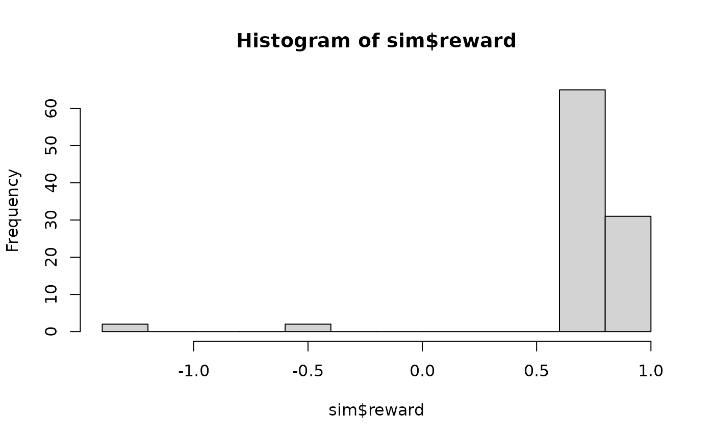
#> $reward
#>   [1]  0.76  0.76  0.84  0.80  0.76  0.84  0.80  0.68  0.76  0.64  0.80  0.68
#>  [13]  0.76  0.76 -0.40  0.80  0.80  0.72  0.64  0.84  0.84  0.84  0.80  0.80
#>  [25]  0.84  0.72  0.80  0.84  0.84  0.68  0.80  0.80  0.84  0.72  0.84  0.72
#>  [37]  0.72  0.76  0.72  0.76  0.84  0.76  0.76  0.80  0.84  0.68  0.84  0.72
#>  [49]  0.84  0.80  0.80  0.80  0.84  0.84  0.84  0.76  0.64  0.84  0.84  0.72
#>  [61]  0.80  0.80  0.72  0.72  0.84  0.76  0.84  0.84  0.76  0.72  0.68  0.72
#>  [73]  0.72  0.64  0.84  0.80  0.68  0.80 -1.24  0.80  0.84  0.84  0.84  0.76
#>  [85]  0.84 -1.24  0.80  0.80  0.76  0.84  0.76  0.76  0.84 -0.40  0.80  0.84
#>  [97]  0.72  0.80  0.76  0.84
#> 
#> $action_cnt
#>    up right  down  left 
#>   279   364     0    16 
#> 
#> $state_cnt
#> s(1,1) s(2,1) s(3,1) s(1,2) s(3,2) s(1,3) s(2,3) s(3,3) s(1,4) s(2,4) s(3,4) 
#>    119    140     26    122     16    124     14      0     96      2      0 
#> 
#> $trajectories
#> data frame with 0 columns and 0 rows
#> 

# Note that all simulations start at s_1 and that the simulated avg. reward
# is therefore an estimate to the U value for the start state s_1.
policy(sol)[1,]
#>    state         U action
#> 1 s(1,1) 0.8513071  right

# Calculate proportion of actions taken in the simulation
round_stochastic(sim$action_cnt / sum(sim$action_cnt), 2)
#>    up right  down  left 
#>  0.42  0.56  0.00  0.02 

# reward distribution
hist(sim$reward)


## Example 2: simulate starting following a uniform distribution over all
#             states and return all trajectories
sim <- simulate_MDP(sol, n = 100, start = "uniform", horizon = 10, 
  return_trajectories = TRUE)
head(sim$trajectories)   
#>   episode time      s    a     r s_prime
#> 1       1    0 s(3,4) left -0.04  s(3,3)
#> 2       1    1 s(3,3) left -0.04  s(2,3)
#> 3       1    2 s(2,3)   up -1.00  s(2,4)
#> 4       2    0 s(1,4) left  0.00  s(1,4)
#> 5       3    0 s(1,4) left  0.00  s(1,4)
#> 6       4    0 s(2,1)   up -0.04  s(2,1)
  
# how often was each state visited?
table(sim$trajectories$s)
#> 
#> s(1,1) s(2,1) s(3,1) s(1,2) s(3,2) s(1,3) s(2,3) s(3,3) s(1,4) s(2,4) s(3,4) 
#>     75     67     58     74     42     86     23     22     10     10      8