Solve MDPs using Dynamic Programming

Solve MDPs via policy and value iteration.

Usage

solve_MDP_DP(
  model,
  method = "VI",
  horizon = NULL,
  discount = NULL,
  n = 1000L,
  error = 0.001,
  k_backups = 10L,
  V = NULL,
  ...,
  matrix = TRUE,
  continue = FALSE,
  verbose = FALSE,
  progress = TRUE
)

Arguments

model

an MDP problem specification.

method

string; one of the following solution methods:

'VI' - value iteration
'PI' - policy iteration
'GenPS', 'PS_error', 'PS_random' - prioritized sweeping

horizon

an integer with the number of epochs for problems with a finite planning horizon. If set to Inf, the algorithm continues running iterations till it converges to the infinite horizon solution. If NULL, then the horizon specified in model will be used.

discount

discount factor in range $(0, 1]$. If NULL, then the discount factor specified in model will be used.

n

maximum number of iterations allowed to converge. If the maximum is reached then the non-converged solution is returned with a warning.

error

value iteration: maximum Bellman error allowed for the convergence criterion.

k_backups

policy iteration: maximum number of Bellman backups used in the iterative policy evaluation step. Policy evaluation typically converges earlier with a maximum Bellman error less than error.

V

a vector with initial state values. If NULL, then the default of a vector of all 0s (V_zero()) is used.

...

further parameters are passed on to the solver function.

matrix

logical; if TRUE then matrices for the transition model and the reward function are taken from the model first. This can be slow if functions need to be converted or do not fit into memory if the models are large. If these components are already matrices, then this is very fast. For FALSE, the transition probabilities and the reward is extracted when needed. This is slower, but removes the time and memory requirements needed to calculate the matrices.

continue

logical; show a progress bar with estimated time for completion.

verbose

logical or a numeric verbose level; if set to TRUE or 1, the function displays the used algorithm parameters and progress information. Levels >1 provide more detailed solver output in the R console.

progress

logical; show a progress bar with estimated time for completion.

Value

solve_MDP() returns an object of class MDP or MDPSample which is a list with the model specifications (model), the solution (solution). The solution is a list with the elements that depend on the used method. Common elements are:

method with the name of the used method
parameters used.
converged did the algorithm converge (NA) for finite-horizon problems.
policy a list representing the policy graph. The list only has one element for converged solutions.

Details

The following dynamic programming methods are implemented using the algorithms presented in Russell and Norvig (2010).

(Modified) Policy Iteration (Howard 1960; Puterman and Shin 1978) starts with a random policy and iteratively performs a sequence of
1. (Approximate) policy evaluation to estimate the value function for the current policy. Iterative policy evaluation can be approximated by stopping early after k_backups iterations (see policy_evaluation(). In this case the algorithm is called modified policy iteration.
2. Policy improvement is performed by updating the policy to be greedy (see greedy_policy()) with respect to the new value function. The algorithm stops when it converges to a stable policy (i.e., no changes between two iterations). Note that the policy typically stabilizes before the value function converges.
Value Iteration (Bellman 1957) starts with an arbitrary value function (by default all 0s) and iteratively updates the value function for each state using the Bellman update equation (see bellman_update()).

$$v(s) \leftarrow \max_{a \in \mathcal{A}(s)} \sum_{s'} p(s' | s,a) [r(s,a, s') + \gamma v(s')]$$

The iteration is terminated when the solution converges or the maximum of n iterations has been reached. Approximate convergence is achieved for discounted problems (with $\gamma < 1$) when the maximal value function change for any state $\delta$ is $$\delta \le \frac{error (1-\gamma)}{\gamma}.$$ It can be shown that this means that no state value is more than $error$ from the value in the optimal value function. For undiscounted problems, we use $\delta \le error$.

A greedy policy is extracted from the final value function. Value iteration can be seen as policy iteration with policy evaluation truncated to one step.
Prioritized Sweeping (Moore and Atkeson, 1993; Andre et al., 1997; Li and Littman, 2008) approximate the optimal value function by iteratively adjusting one state at a time. While value and policy iteration sweep in every iteration through all states, prioritized sweeping updates states in the order given by their priority. The priority reflects how much a state value may change given the most recently updated other states that can be directly reached via an action. This update order often lead to faster convergence compared to sweeping the whole state space in regular value iteration.

We implement the two priority update strategies described as PS and GenPS by Li and Littman (2008).
- PS (Moore and Atkeson, 1993) updates the priority of a state $H(s)$ using: $$ \forall{s \in \mathcal{S}}: H_{t+1}(s) \leftarrow \begin{cases} \max(H_{t}(s), \Delta_t \max_{a \in \mathcal{A}}(p(s_t|s,a)) \text{ for } s \ne s_{t+1} \\ \Delta_t \max_{a \in A}(p(s_t|s,a) \text{ for } s = s_{t+1} \end{cases} $$
  
  where $\Delta_t = |V_{t+1}(s_t) - V_t(s_t)| = |E(s_t; V_{t+1})|$, i.e., the Bellman error for the updated state.
- GenPS (Andre et al., 1997) updates all state priorities using their current Bellman error:
  
  $$\forall{s \in \mathcal{S}}: H_{t+1}(s) \leftarrow |E(s; V_{t+1})|$$
  
  where $E(s; V_{t+1}) = \max_{a \in A} \left[R(s,a) + \gamma \sum_{s \in S} p(s'|s,a) V(s')\right] - V(s)$ is a state's Bellman error.
The update method can be chosen using the additional parameter H_update as the character string "PS_random", "PS_error" or "GenPS". The default is H_update = "GenPS". For PS, random means that the priority vector is initialized with random values (larger than 0), and error means they are initialized with the Bellman error as in GenPS. However, this requires one complete sweep over all states.

This implementation stops updating when the largest priority values over all states is less than the specified error.

Since the algorithm does not sweep through the whole state space for each iteration, n is converted into an equivalent number of state updates $n = n\ |S|$.

References

Andre, D., Friedman, N., and Parr, R. 1997. "Generalized prioritized sweeping." In Advances in Neural Information Processing Systems 10, pp. 1001-1007. NeurIPS Proceedings

Bellman, Richard. 1957. "A Markovian Decision Process." Indiana University Mathematics Journal 6: 679-84. https://www.jstor.org/stable/24900506.

Howard, R. A. 1960. "Dynamic Programming and Markov Processes." Cambridge, MA: MIT Press.

Li, Lihong, and Michael Littman. 2008. "Prioritized Sweeping Converges to the Optimal Value Function." DCS-TR-631. Rutgers University. doi:10.7282/T3TX3JSX

Moore, Andrew, and C. G. Atkeson. 1993. "Prioritized Sweeping: Reinforcement Learning with Less Data and Less Real Time." Machine Learning 13 (1): 103–30. doi:10.1007/BF00993104 .

Puterman, Martin L., and Moon Chirl Shin. 1978. "Modified Policy Iteration Algorithms for Discounted Markov Decision Problems." Management Science 24: 1127-37. doi:10.1287/mnsc.24.11.1127 .

Russell, Stuart J., and Peter Norvig. 2020. Artificial Intelligence: A Modern Approach (4th Edition). Pearson. http://aima.cs.berkeley.edu/.

Examples

data(Maze)

maze_solved <- solve_MDP(Maze, method = "DP:VI", verbose = TRUE)
#> Precomputing matrices for R and T ... done.
#> Running value iteration (infinite horizon)
#> error for convergence:   0.001
#> n (max iterations):      1000
#> Initial V (first 20 max):
#> s(1,1) s(2,1) s(3,1) s(1,2) s(3,2) s(1,3) s(2,3) s(3,3) s(1,4) s(2,4) s(3,4) 
#>      0      0      0      0      0      0      0      0      0      0      0 
#> 
#> Terminated at iteration: 19 
policy(maze_solved)
#>     state         V action
#> 1  s(1,1) 0.8115564  right
#> 2  s(2,1) 0.7615521     up
#> 3  s(3,1) 0.7052527     up
#> 4  s(1,2) 0.8678082  right
#> 5  s(3,2) 0.6551492   left
#> 6  s(1,3) 0.9178082  right
#> 7  s(2,3) 0.6602740     up
#> 8  s(3,3) 0.6110843   left
#> 9  s(1,4) 0.0000000     up
#> 10 s(2,4) 0.0000000  right
#> 11 s(3,4) 0.3872455   left

# use prioritized sweeping (which is known to be fast for mazes)
maze_solved <- solve_MDP(Maze, method = "DP:GenPS", verbose = TRUE)
#> Precomputing matrices for R and T ... done.
#> Running prioritized sweeping
#> H_update:               GenPS
#> error for convergence:  0.001
#> n (max updates):        11000
#> Initial V (first 20 max):
#>  [1] -0.04 -0.04 -0.04 -0.04 -0.04  0.76 -0.04 -0.04  0.00  0.00 -0.04
#> 
#> State updates performed: 89 (equivalent to 8.09 complete sweeps) 
#> Converged: TRUE 
policy(maze_solved)
#>     state         V action
#> 1  s(1,1) 0.8104998  right
#> 2  s(2,1) 0.7600309     up
#> 3  s(3,1) 0.7030110     up
#> 4  s(1,2) 0.8672276  right
#> 5  s(3,2) 0.6522679   left
#> 6  s(1,3) 0.9174998  right
#> 7  s(2,3) 0.6598484     up
#> 8  s(3,3) 0.6083265   left
#> 9  s(1,4) 0.0000000   down
#> 10 s(2,4) 0.0000000  right
#> 11 s(3,4) 0.3848524   left

# finite horizon
maze_solved <- solve_MDP(Maze, method = "DP:VI", horizon = 3)
policy(maze_solved)
#> [[1]]
#>     state       V action
#> 1  s(1,1)  0.3920  right
#> 2  s(2,1) -0.1200     up
#> 3  s(3,1) -0.1200  right
#> 4  s(1,2)  0.7376  right
#> 5  s(3,2) -0.1200   down
#> 6  s(1,3)  0.8896  right
#> 7  s(2,3)  0.5720     up
#> 8  s(3,3)  0.3152     up
#> 9  s(1,4)  0.0000     up
#> 10 s(2,4)  0.0000     up
#> 11 s(3,4) -0.1200   down
#> 
#> [[2]]
#>     state      V action
#> 1  s(1,1) -0.080  right
#> 2  s(2,1) -0.080     up
#> 3  s(3,1) -0.080  right
#> 4  s(1,2)  0.560  right
#> 5  s(3,2) -0.080   left
#> 6  s(1,3)  0.832  right
#> 7  s(2,3)  0.464     up
#> 8  s(3,3) -0.080   left
#> 9  s(1,4)  0.000     up
#> 10 s(2,4)  0.000     up
#> 11 s(3,4) -0.080   down
#> 
#> [[3]]
#>     state     V action
#> 1  s(1,1) -0.04  right
#> 2  s(2,1) -0.04     up
#> 3  s(3,1) -0.04  right
#> 4  s(1,2) -0.04  right
#> 5  s(3,2) -0.04  right
#> 6  s(1,3)  0.76  right
#> 7  s(2,3) -0.04   left
#> 8  s(3,3) -0.04  right
#> 9  s(1,4)  0.00   left
#> 10 s(2,4)  0.00     up
#> 11 s(3,4) -0.04   down
#> 
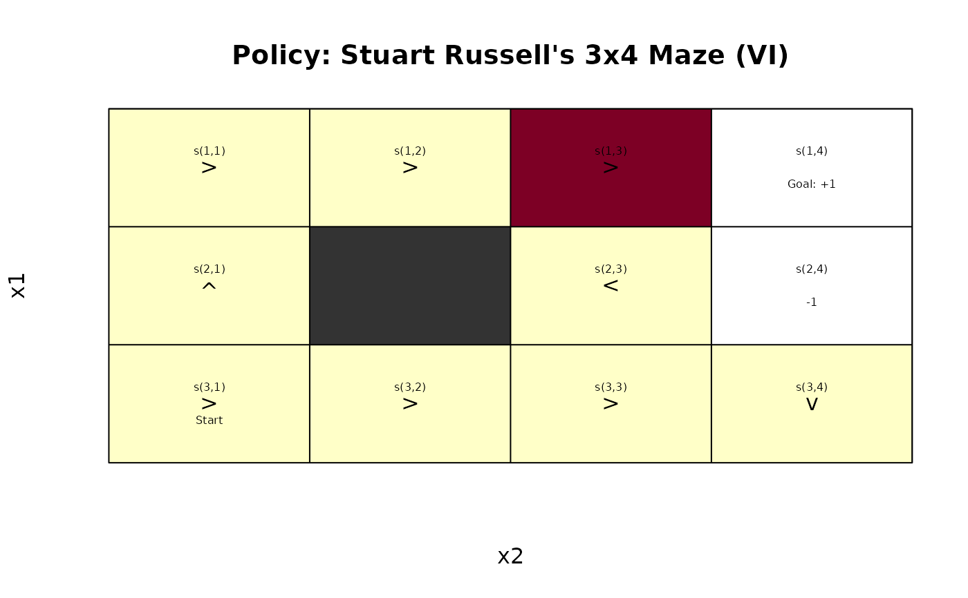
gw_plot(maze_solved, epoch = 1)

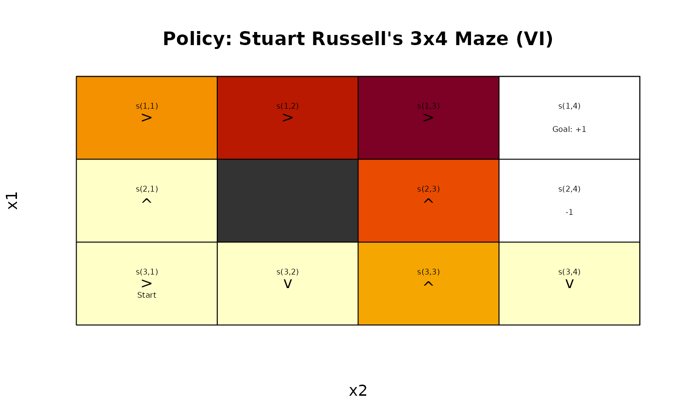gw_plot(maze_solved, epoch = 2)

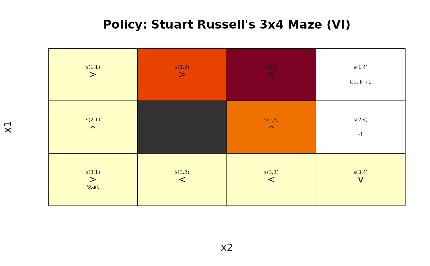gw_plot(maze_solved, epoch = 3)