Schedules to Reduce Alpha, Epsilon and Other Parameters

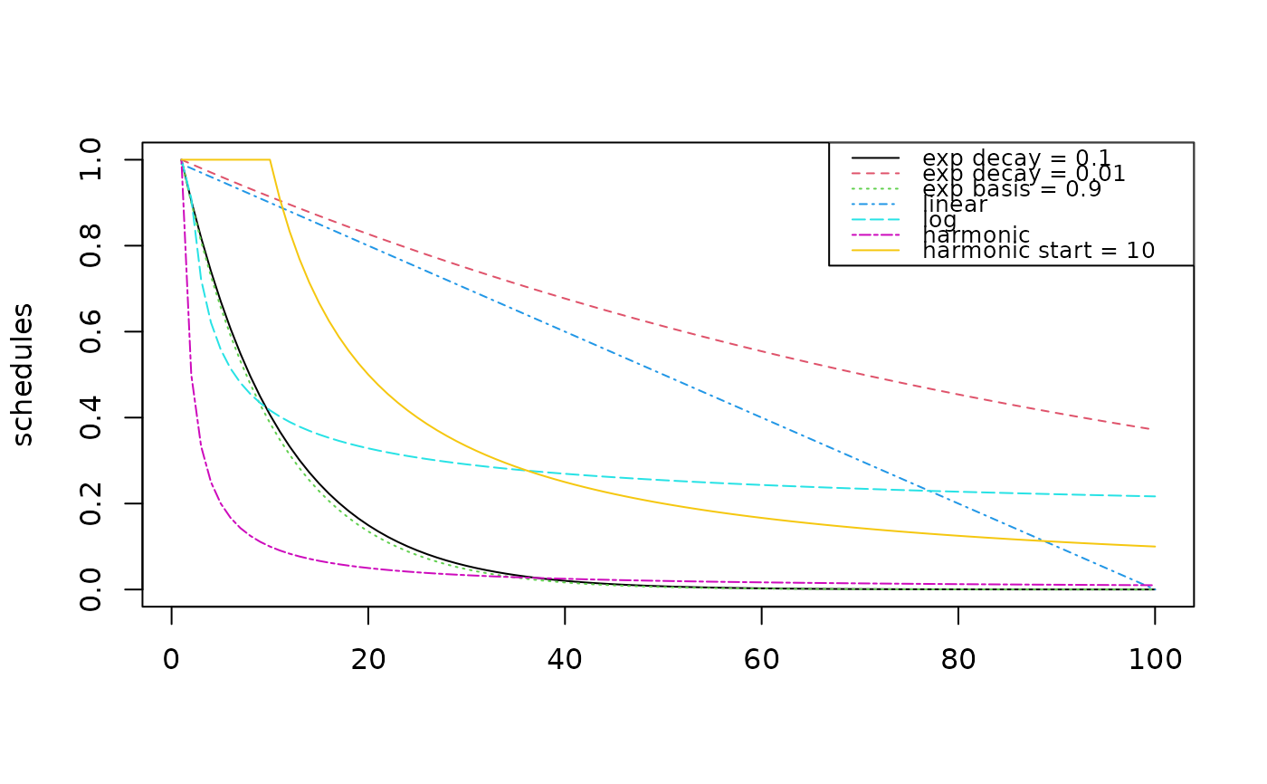
Several schedule functions to reduce learning parameters are available using generator functions.

Usage

schedule_exp(start, decay)

schedule_exp2(start, basis)

schedule_log(start)

schedule_linear(start, end, n)

schedule_harmonic(start, n)

Arguments

start

start value for the schedule.

decay

decay factor for exponential schedules.

basis

basis for exponential schedules.

end

end value for the schedule.

n

number of steps (e.g., epochs) for the schedule.

Details

Several learning parameters need to be reduced during learning to ensure convergence. We provide several schedule function generators that reduce learning parameters after each processed episode or according to the number of times a state-action combination was tried.

Here are the definitions of the available schedules:

• schedule_exp : function(t) start * exp(-decay * (t - 1))

• schedule_exp2 : function(t) start * basis^(t - 1)

• schedule_log : function(t) pmin(start/log(1 + t), start)

• schedule_linear : step <- (start - end)/n function(t) start - t * step

• schedule_harmonic : function(t) pmin(start/t, 1)

t is the time step, episode number or count starting with 1.

See also

Other solver: convergence_horizon(), solve_MDP(), solve_MDP_APPROX(), solve_MDP_DP(), solve_MDP_LP(), solve_MDP_MC(), solve_MDP_PG(), solve_MDP_SAMP(), solve_MDP_TD()

Examples

# create an exponential  schedule function
s_exp <- schedule_exp(1, decay = .1)
s_exp
#> function (t) 
#> start * exp(-decay * (t - 1))
#> <bytecode: 0x55fb69e5e8b8>
#> <environment: 0x55fb6c0c4328>

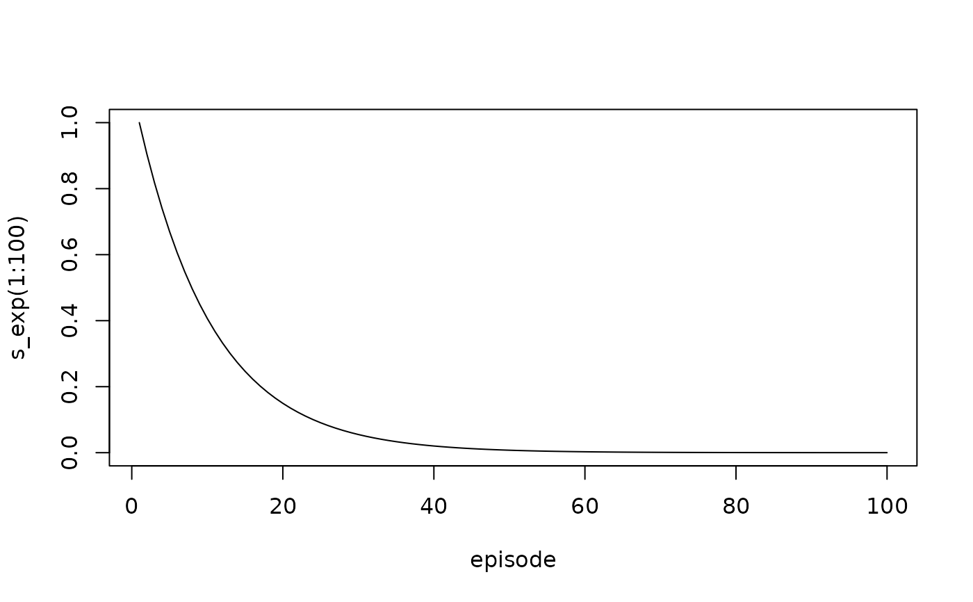
# plot the schedule for 100 episodes.
episode <- seq_len(100)
plot(x = episode, s_exp(1:100), type = "l")


# compare some schedule examples
schedules <- cbind(
  `exp decay = 0.1` = schedule_exp(1, decay = .1)(1:100),
  `exp decay = 0.01` = schedule_exp(1, decay = .01)(1:100),
  `exp basis = 0.9` = schedule_exp2(1, basis = .9)(1:100),
  `linear` = schedule_linear(1, end = 0, n = 100)(1:100),
  `log` = schedule_log(1)(1:100),
  `harmonic` = schedule_harmonic(1, n = 100)(1:100),
  `harmonic start = 10` = schedule_harmonic(10, n = 100)(1:100)
  )
 
matplot(schedules, type = "l", 
        col = 1:ncol(schedules),
        lty = 1:ncol(schedules)
        )
legend("topright", 
        legend = colnames(schedules), 
        col = 1:ncol(schedules), 
        lty = 1:ncol(schedules),
        cex = 0.8
        )