Implementation of value iteration, modified policy iteration and other methods based on reinforcement learning techniques to solve finite state space MDPs.
Usage
solve_MDP(model, ...)

# S3 method for class 'MDP'
solve_MDP(
  model,
  method = "DP:VI",
  horizon = NULL,
  discount = NULL,
  ...,
  matrix = TRUE,
  continue = FALSE,
  verbose = FALSE,
  progress = !verbose
)

# S3 method for class 'MDPSample'
solve_MDP(
  model,
  method = "APPROX:semi_gradient_sarsa",
  horizon = NULL,
  discount = NULL,
  ...,
  matrix = TRUE,
  continue = FALSE,
  verbose = FALSE,
  progress = !verbose
)
Arguments
- model
an MDP problem specification.
- ...
further parameters are passed on to the solver function.
- method
string; Composed of the algorithm family abbreviation and the algorithm separated by
:. The algorithm families can be found in the See Also section under "Other solvers". The family abbreviation followssolve_MDP_in the function name.- horizon
an integer with the number of epochs for problems with a finite planning horizon. If set to
Inf, the algorithm continues running iterations till it converges to the infinite horizon solution. IfNULL, then the horizon specified inmodelwill be used.- discount
discount factor in range \((0, 1]\). If
NULL, then the discount factor specified inmodelwill be used.- matrix
logical; if
TRUEthen matrices for the transition model and the reward function are taken from the model first. This can be slow if functions need to be converted or do not fit into memory if the models are large. If these components are already matrices, then this is very fast. ForFALSE, the transition probabilities and the reward is extracted when needed. This is slower, but removes the time and memory requirements needed to calculate the matrices.- continue
logical; show a progress bar with estimated time for completion.
- verbose
logical or a numeric verbose level; if set to
TRUEor1, the function displays the used algorithm parameters and progress information. Levels>1provide more detailed solver output in the R console.- progress
logical; show a progress bar with estimated time for completion.
Value
solve_MDP() returns an object of class MDP or MDPSample which is a list with the
model specifications (model), the solution (solution).
The solution is a list with the elements that depend on the used method. Common
elements are:
methodwith the name of the used methodparameters used.
convergeddid the algorithm converge (NA) for finite-horizon problems.policya list representing the policy graph. The list only has one element for converged solutions.
Details
Several solvers are available. Note that some solvers are only implemented for finite-horizon problems.
Most solvers can be interrupted using Esc/CTRL-C and will return the
current solution. Solving can be continued by calling solve_MDP with the
partial solution as the model and the parameter continue = TRUE. This method
can also be used to reduce parameters like alpha or epsilon (see Q-learning
in the Examples section).
A list of available solvers can be found in the See Also section under "Other solvers".
While MDP model contain an explicit specification of the state space,
the transition probabilities and the reward structure, MDPSample only contains a
transition function. This means that only a small subset of solvers can be
used for MDPSamples. This currently includes only includes
the solvers in solve_MDP_APPROX().
References
Russell, Stuart J., and Peter Norvig. 2020. Artificial Intelligence: A Modern Approach (4th Edition). Pearson. http://aima.cs.berkeley.edu/.
Sutton, Richard S., and Andrew G. Barto. 2018. Reinforcement Learning: An Introduction. Second. The MIT Press. http://incompleteideas.net/book/the-book-2nd.html.
Examples
data(Maze)
Maze
#> MDPModel, MDP - Stuart Russell's 3x4 Maze
#> Discount factor: 1
#> Horizon: Inf epochs
#> Size: 4 actions / 11 states
#> Storage: transition prob as matrix / reward as matrix. Total size: 28.8 Kb
#> Start: s(3,1)
#> Model list components: ‘name’, ‘discount’, ‘horizon’, ‘states’,
#> ‘actions’, ‘start’, ‘transition_model’, ‘reward’, ‘info’,
#> ‘absorbing_states’
# default is value iteration (VI)
maze_solved <- solve_MDP(Maze)
maze_solved
#> MDPModel, MDP - Stuart Russell's 3x4 Maze
#> Discount factor: 1
#> Horizon: Inf epochs
#> Size: 4 actions / 11 states
#> Storage: transition prob as matrix / reward as matrix. Total size: 32.3 Kb
#> Start: s(3,1)
#> Model list components: ‘name’, ‘discount’, ‘horizon’, ‘states’,
#> ‘actions’, ‘start’, ‘transition_model’, ‘reward’, ‘info’,
#> ‘absorbing_states’, ‘solution’
#>
#> Solved:
#> Method: ‘VI’
#> Solution converged: TRUE
#> Solution list components: ‘method’, ‘policy’, ‘converged’, ‘delta’,
#> ‘iterations’
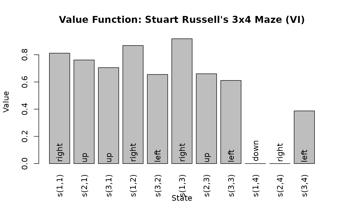
policy(maze_solved)
#> state V action
#> 1 s(1,1) 0.8115564 right
#> 2 s(2,1) 0.7615521 up
#> 3 s(3,1) 0.7052527 up
#> 4 s(1,2) 0.8678082 right
#> 5 s(3,2) 0.6551492 left
#> 6 s(1,3) 0.9178082 right
#> 7 s(2,3) 0.6602740 up
#> 8 s(3,3) 0.6110843 left
#> 9 s(1,4) 0.0000000 down
#> 10 s(2,4) 0.0000000 right
#> 11 s(3,4) 0.3872455 left
# plot the value function U
plot_value_function(maze_solved)
 # Gridworld solutions can be visualized
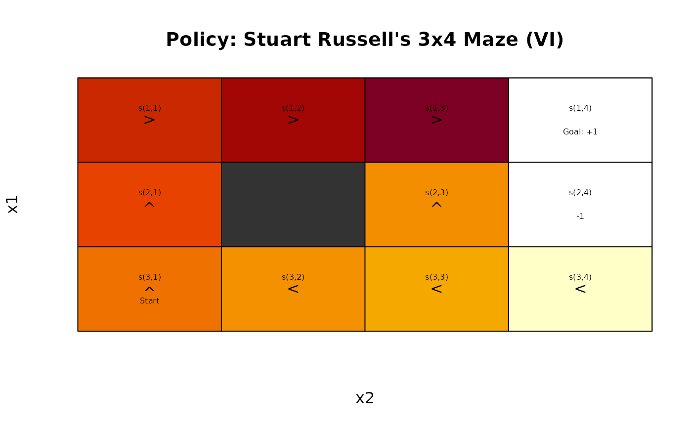
gw_plot(maze_solved)
# Gridworld solutions can be visualized
gw_plot(maze_solved)