Define an MDP With Only Sample Access

Defines a discrete-time Markov decision process with only sample access as a transition function between states using a factored state representation. The state space may be continuous and infinite.

Usage

MDPSample(
  actions,
  transition_model,
  start,
  states = NULL,
  absorbing_states = NULL,
  discount = 0.9,
  horizon = Inf,
  info = NULL,
  name = NA
)

Arguments

actions: a character vector specifying the names of the available actions.
transition_model: A transition function receiving the current state features and returning the reward and the next state features.
start: Specifies in which state the MDP starts.
states: Optional state labels.
absorbing_states: a single state or a list with absorbing states.
discount: numeric; discount rate between 0 and 1.
horizon: numeric; Number of epochs.
info: A list with additional information.
name: a string to identify the MDP problem.

Value

The function returns an object of class MDPSample which is list with the model specification.

Details

Defines a Markov decision process as a transition function between state represented as feature vectors (i.e., using a factored state representation). The state space may be

finite and discrete and specified in the problem,
finite and discrete but not specified in the problem,
continuous (implying infinite and not specified in the problem).

Compared to the specification in class MDP, no transition probabilities are available. Instead of the reward function, reward is only returned from calls to the transition function via act(). The state space may be specified.

To represent states, a factored state representation as a row vector for a single state or a matrix with row vectors for a set of states are used. State labels can be constructed in the form s(feature1, feature2, ...). Conversion between the factored representation and state labels is available in state2features() and features2state(). Since the state set is not directly represented, state ids cannot be used!

Reinforcement learning algorithms with approximation can be used to solve these problems. See: solve_MDP_APPROX().

Author

Michael Hahsler

Examples

# Example 1: Define a simple 5x5 maze without walls

transition_model <- function(model, action, state) {
  # make sure action and state are in the correct format
  action <- normalize_action_label(action, model)
  state <- normalize_state_features(state, model)
  
  if (all(state == s(5, 5)))
    return(list(reward = 0, state_prime = state))

  sp <- state + switch(action,
    up =   c( -1, 0),
    down = c( +1, 0),
    left = c(  0,-1),
    right = c( 0,+1)
  )
  r <- -1

  # check bounds
  if (any(sp < 1) || any(sp > 5)) {
      sp <- state
   }

  # goal
  if (all(sp == s(5, 5)))
    r <- 100

  return(list(reward = r, state_prime = sp))
}

m <- MDPSample(actions = c("up", "right", "down", "left"),
          transition_model,
          start = s(1,1),
          absorbing_states = s(5, 5),
          name = "5x5 Maze")
m
#> MDPSample, MDP - 5x5 Maze
#>   Discount factor: 0.9
#>   Horizon: Inf epochs
#>   Size: 4 actions / undefined state space
#>   Start: s(1,1)
#>   List components: ‘name’, ‘discount’, ‘horizon’, ‘actions’, ‘states’,
#>     ‘start’, ‘absorbing_states’, ‘transition_model’, ‘info’

act(m, s(1,1), "down")
#> $reward
#> [1] -1
#> 
#> $state_prime
#>      x1 x2
#> [1,]  2  1
#> 

# Reach the goal: reward = 100
act(m, s(5,4), "right")
#> $reward
#> [1] 100
#> 
#> $state_prime
#>      x1 x2
#> [1,]  5  5
#> 

# Illegal action: no movement and reward = -1
act(m, s(1,1), "up")
#> $reward
#> [1] -1
#> 
#> $state_prime
#>      x1 x2
#> [1,]  1  1
#> 

# Absorbing state: no movement and 0 reward
act(m, s(5,5), "up")
#> $reward
#> [1] 0
#> 
#> $state_prime
#>      x1 x2
#> [1,]  5  5
#> 


# Example 2: Solve using Linear Feature Approximation

# Note that we have not specified the state space
m
#> MDPSample, MDP - 5x5 Maze
#>   Discount factor: 0.9
#>   Horizon: Inf epochs
#>   Size: 4 actions / undefined state space
#>   Start: s(1,1)
#>   List components: ‘name’, ‘discount’, ‘horizon’, ‘actions’, ‘states’,
#>     ‘start’, ‘absorbing_states’, ‘transition_model’, ‘info’
S(m)
#> NULL

# To use value function approximation, we need to specify the minimum
# and maximum of each state feature for scaling them to [0,1]. The rows
# and column indices used are between 0 and 5.
set.seed(1000)
sol <- solve_MDP_APPROX(m, horizon = 1000, n = 100,
          alpha = 0.01, epsilon = 0.55, 
          transformation = transformation_linear_basis, 
          min = c(0, 0), max = c(5, 5),
          verbose = FALSE)

# we can calculate the approximate q-values, but have to specify the states.
approx_Q_value(sol, state = rbind(s(1,2), s(4,5)))
#>            up    right     down     left
#> [1,] 12.99841 17.82052 17.37264 12.43688
#> [2,] 20.61977 36.13659 34.90891 19.84653

# Note: since there is no explicit state space, we also do not have a 
#       precalculated policy! We can get approx. greedy actions.

approx_greedy_action(sol, state = s(4,5))
#> [1] right
#> Levels: up right down left
 
# Example 3: MDPSample with a specified state space  

# The same maze as above can be created with this gridworld helper.
# It specifies the finite state space.
m <- gw_maze_MDP(dim = c(5,5), start = "s(1,1)", goal = "s(5,5)", access = "sample")
m
#> MDPSample, MDP - A Maze
#>   Discount factor: 1
#>   Horizon: Inf epochs
#>   Size: 4 actions / 25 states
#>   Start: s(1,1)
#>   List components: ‘name’, ‘discount’, ‘horizon’, ‘actions’, ‘states’,
#>     ‘start’, ‘absorbing_states’, ‘transition_model’, ‘info’
S(m)
#>  [1] "s(1,1)" "s(2,1)" "s(3,1)" "s(4,1)" "s(5,1)" "s(1,2)" "s(2,2)" "s(3,2)"
#>  [9] "s(4,2)" "s(5,2)" "s(1,3)" "s(2,3)" "s(3,3)" "s(4,3)" "s(5,3)" "s(1,4)"
#> [17] "s(2,4)" "s(3,4)" "s(4,4)" "s(5,4)" "s(1,5)" "s(2,5)" "s(3,5)" "s(4,5)"
#> [25] "s(5,5)"

# With the defined state space, we do not need to supply min and max 
# for the transformation function.
set.seed(1000)
sol <- solve_MDP_APPROX(m, horizon = 1000, n = 100,
          alpha = 0.01, epsilon = 0.55, verbose = FALSE)

# we can use several gridworld helper
gw_plot(sol)

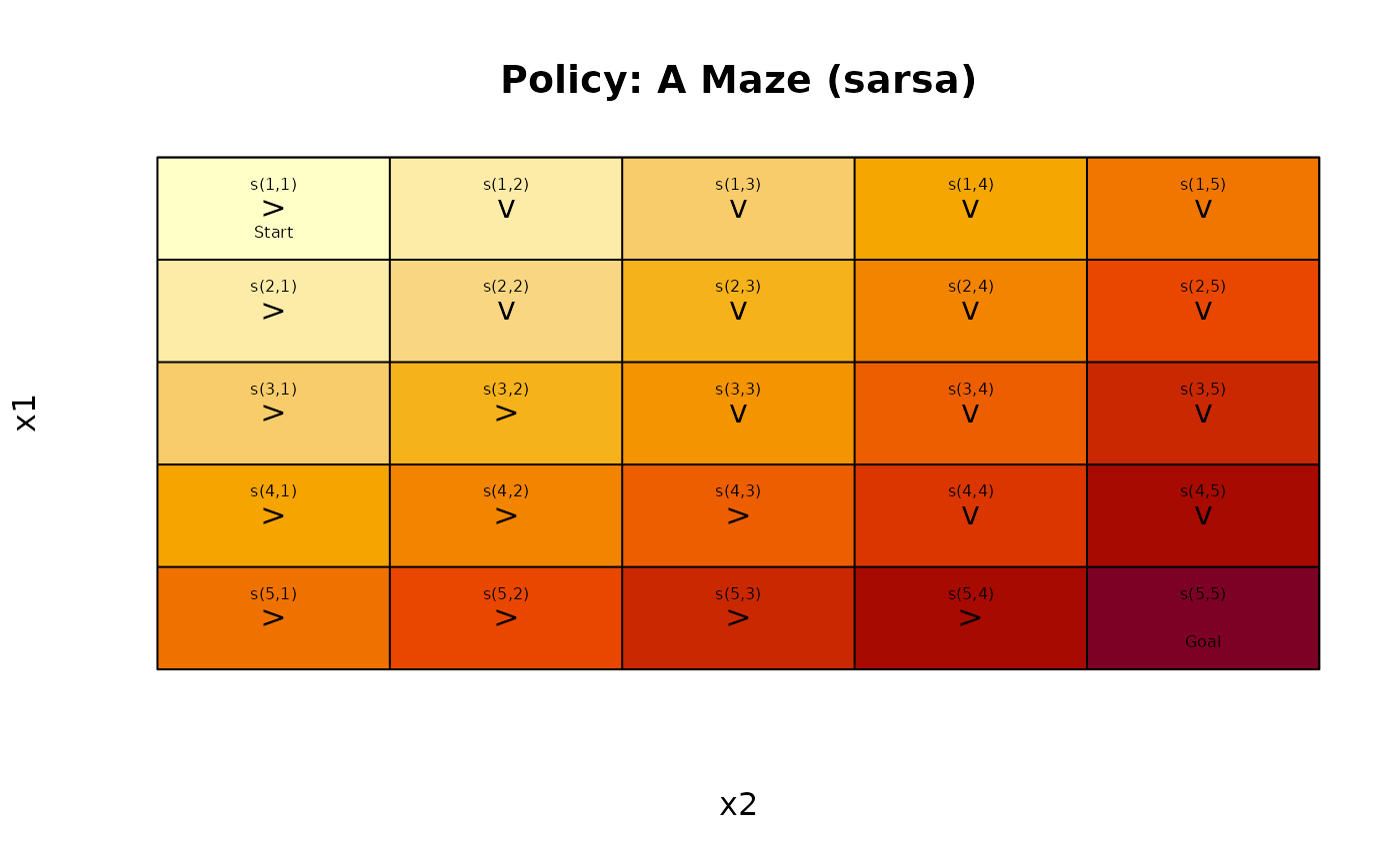gw_matrix(sol, what = "value")
#>          [,1]     [,2]     [,3]     [,4]     [,5]
#> [1,] 18.35811 24.21770 30.14518 36.07267 42.00015
#> [2,] 24.37361 28.37248 34.29996 40.22745 46.15493
#> [3,] 30.38912 34.32785 38.45474 44.38222 50.30971
#> [4,] 36.40462 40.34335 44.28208 48.53700 54.46449
#> [5,] 42.42012 46.35885 50.29758 54.23631 58.61927

# and get a policy table
policy(sol)
#>     state        V action
#> 1  s(1,1) 18.35811  right
#> 2  s(2,1) 24.37361  right
#> 3  s(3,1) 30.38912  right
#> 4  s(4,1) 36.40462  right
#> 5  s(5,1) 42.42012  right
#> 6  s(1,2) 24.21770   down
#> 7  s(2,2) 28.37248   down
#> 8  s(3,2) 34.32785  right
#> 9  s(4,2) 40.34335  right
#> 10 s(5,2) 46.35885  right
#> 11 s(1,3) 30.14518   down
#> 12 s(2,3) 34.29996   down
#> 13 s(3,3) 38.45474   down
#> 14 s(4,3) 44.28208  right
#> 15 s(5,3) 50.29758  right
#> 16 s(1,4) 36.07267   down
#> 17 s(2,4) 40.22745   down
#> 18 s(3,4) 44.38222   down
#> 19 s(4,4) 48.53700   down
#> 20 s(5,4) 54.23631  right
#> 21 s(1,5) 42.00015   down
#> 22 s(2,5) 46.15493   down
#> 23 s(3,5) 50.30971   down
#> 24 s(4,5) 54.46449   down
#> 25 s(5,5) 58.61927   down