3 Classification: Basic Concepts
This chapter introduces decision trees for classification and discusses how models are built and evaluated.
3.1 Learning Objectives
After this chapter, you should be able to:
- train and interpret a decision tree classifier;
- distinguish training, validation, and test data;
- tune model hyperparameters without using the test set; and
- evaluate classification performance with a confusion matrix and suitable metrics.
3.2 Prerequisites
Read Introduction and Data. Basic familiarity with R formulas, factors, probability, and summary statistics is assumed.
The corresponding chapter of the data mining textbook is available online: Chapter 3: Classification: Basic Concepts and Techniques.
Packages Used in this Chapter
pkgs <- c("basemodels", "caret", "FSelector", "lattice", "mlbench",
          "palmerpenguins", "party", "pROC", "rpart",
          "rpart.plot", "tidyverse")

pak::pkg_install(pkgs)
The packages used for this chapter are:
- basemodels (Chen et al. 2023)
- caret (Kuhn 2024)
- FSelector (Romanski, Kotthoff, and Schratz 2023)
- lattice (Sarkar 2026)
- mlbench (Leisch and Dimitriadou 2026)
- palmerpenguins (Horst, Hill, and Gorman 2022)
- party (Hothorn et al. 2026)
- pROC (Robin et al. 2026)
- rpart (Therneau and Atkinson 2026)
- rpart.plot (Milborrow 2026)
- tidyverse (Wickham 2023)
This book uses caret for the classification
workflows in its examples, including resampling, tuning, and evaluation. Model
algorithms are supplied by their own R packages. tidymodels
is a separate R modeling framework and is not used in this book; its workflows
are not interchangeable line-for-line with caret.
3.3 Basic Concepts
Classification is a machine learning task with the goal to learn a predictive function of the form
\[y = f(\mathbf{x}),\]
where \(\mathbf{x}\) is the feature vector and \(y\) is the class label. The features describe an object and may be measured on different scales (for example, nominal or numeric). The class label is categorical. If it has two possible values, the task is binary classification.
Classification learns a model from training data containing both features and their known labels. It is therefore a supervised learning problem.
A related supervised learning problem is regression, where \(y\) is a number instead of a label. Linear regression is a very popular supervised learning model which is taught in almost any introductory statistics course. Code examples for regression are available in the extra Chapter Regression.
This chapter will introduce decision trees, model evaluation and comparison, feature selection, and then explore methods to handle the class imbalance problem.
You can read the free sample chapter from the textbook (Tan, Steinbach, and Kumar 2005): Chapter 3. Classification: Basic Concepts and Techniques
3.4 General Framework for Classification
Supervised learning has two steps:
- Induction: Training a model on training data with known class labels.
- Deduction: Predicting class labels for new data.
We evaluate a model by predicting classes for observations whose labels are known, then comparing the predictions with those labels. When the observations were not used to fit the model, they form test data. Measuring performance on the training data gives the resubstitution error; this is not a reliable estimate of performance on new data because the model was fitted to those same observations.
We typically want to estimate how well the model generalizes to new data, so the test data and training data do not overlap. Error measured on a test set estimates the model’s generalization error.
This chapter builds up the needed concepts. A complete example of how to perform model selection and estimate the generalization error is in the section Hyperparameter Tuning.
3.4.1 The Zoo Dataset
To demonstrate classification, we will use the Zoo dataset which is included in the R package mlbench (you may have to install it). The Zoo dataset containing 17 (mostly logical) variables for 101 animals as a data frame with 17 columns (hair, feathers, eggs, milk, airborne, aquatic, predator, toothed, backbone, breathes, venomous, fins, legs, tail, domestic, catsize, type). The first 16 columns represent the feature vector \(\mathbf{x}\) and the last column called type is the class label \(y\). We convert the data frame into a tidyverse tibble (optional).
data(Zoo, package="mlbench")
head(Zoo)
##           hair feathers  eggs  milk airborne aquatic
## aardvark  TRUE    FALSE FALSE  TRUE    FALSE   FALSE
## antelope  TRUE    FALSE FALSE  TRUE    FALSE   FALSE
## bass     FALSE    FALSE  TRUE FALSE    FALSE    TRUE
## bear      TRUE    FALSE FALSE  TRUE    FALSE   FALSE
## boar      TRUE    FALSE FALSE  TRUE    FALSE   FALSE
## buffalo   TRUE    FALSE FALSE  TRUE    FALSE   FALSE
##          predator toothed backbone breathes venomous  fins
## aardvark     TRUE    TRUE     TRUE     TRUE    FALSE FALSE
## antelope    FALSE    TRUE     TRUE     TRUE    FALSE FALSE
## bass         TRUE    TRUE     TRUE    FALSE    FALSE  TRUE
## bear         TRUE    TRUE     TRUE     TRUE    FALSE FALSE
## boar         TRUE    TRUE     TRUE     TRUE    FALSE FALSE
## buffalo     FALSE    TRUE     TRUE     TRUE    FALSE FALSE
##          legs  tail domestic catsize   type
## aardvark    4 FALSE    FALSE    TRUE mammal
## antelope    4  TRUE    FALSE    TRUE mammal
## bass        0  TRUE    FALSE   FALSE   fish
## bear        4 FALSE    FALSE    TRUE mammal
## boar        4  TRUE    FALSE    TRUE mammal
## buffalo     4  TRUE    FALSE    TRUE mammal
Note: data.frames in R can have row names. The Zoo data set uses the
animal name as the row names. tibbles from tidyverse do not support
row names. To keep the animal name you can add a column with the animal
name.
library(tidyverse)
## ── Attaching core tidyverse packages ──── tidyverse 2.0.0 ──
## ✔ dplyr     1.2.1     ✔ readr     2.2.0
## ✔ forcats   1.0.1     ✔ stringr   1.6.0
## ✔ ggplot2   4.0.3     ✔ tibble    3.3.1
## ✔ lubridate 1.9.5     ✔ tidyr     1.3.2
## ✔ purrr     1.2.2
## ── Conflicts ────────────────────── tidyverse_conflicts() ──
## ✖ dplyr::filter() masks stats::filter()
## ✖ dplyr::lag()    masks stats::lag()
## ℹ Use the conflicted package (<http://conflicted.r-lib.org/>) to force all conflicts to become errors
Zoo <- as_tibble(Zoo, rownames = "animal")
Zoo
## # A tibble: 101 × 18
##    animal   hair  feathers eggs  milk  airborne aquatic
##    <chr>    <lgl> <lgl>    <lgl> <lgl> <lgl>    <lgl>
##  1 aardvark TRUE  FALSE    FALSE TRUE  FALSE    FALSE
##  2 antelope TRUE  FALSE    FALSE TRUE  FALSE    FALSE
##  3 bass     FALSE FALSE    TRUE  FALSE FALSE    TRUE
##  4 bear     TRUE  FALSE    FALSE TRUE  FALSE    FALSE
##  5 boar     TRUE  FALSE    FALSE TRUE  FALSE    FALSE
##  6 buffalo  TRUE  FALSE    FALSE TRUE  FALSE    FALSE
##  7 calf     TRUE  FALSE    FALSE TRUE  FALSE    FALSE
##  8 carp     FALSE FALSE    TRUE  FALSE FALSE    TRUE
##  9 catfish  FALSE FALSE    TRUE  FALSE FALSE    TRUE
## 10 cavy     TRUE  FALSE    FALSE TRUE  FALSE    FALSE
## # ℹ 91 more rows
## # ℹ 11 more variables: predator <lgl>, toothed <lgl>,
## #   backbone <lgl>, breathes <lgl>, venomous <lgl>,
## #   fins <lgl>, legs <int>, tail <lgl>, domestic <lgl>,
## #   catsize <lgl>, type <fct>
You will have to remove the animal column before learning a model since it is a unique identifier!
I translate all the TRUE/FALSE values into factors (nominal). This is
often needed for building models. Always check summary() to make sure
the data is ready for model learning.
Zoo <- Zoo |>
  mutate(across(where(is.logical),
         function (x) factor(x, levels = c(TRUE, FALSE)))) |>
  mutate(across(where(is.character), factor))

summary(Zoo)
##       animal      hair     feathers     eggs       milk
##  aardvark: 1   TRUE :43   TRUE :20   TRUE :59   TRUE :41
##  antelope: 1   FALSE:58   FALSE:81   FALSE:42   FALSE:60
##  bass    : 1
##  bear    : 1
##  boar    : 1
##  buffalo : 1
##  (Other) :95
##   airborne   aquatic    predator   toothed    backbone
##  TRUE :24   TRUE :36   TRUE :56   TRUE :61   TRUE :83
##  FALSE:77   FALSE:65   FALSE:45   FALSE:40   FALSE:18
##
##
##
##
##
##   breathes   venomous     fins         legs         tail
##  TRUE :80   TRUE : 8   TRUE :17   Min.   :0.00   TRUE :75
##  FALSE:21   FALSE:93   FALSE:84   1st Qu.:2.00   FALSE:26
##                                   Median :4.00
##                                   Mean   :2.84
##                                   3rd Qu.:4.00
##                                   Max.   :8.00
##
##   domestic   catsize              type
##  TRUE :13   TRUE :44   mammal       :41
##  FALSE:88   FALSE:57   bird         :20
##                        reptile      : 5
##                        fish         :13
##                        amphibian    : 4
##                        insect       : 8
##                        mollusc.et.al:10
3.5 Decision Tree Classifiers
We use rpart, an implementation of recursive partitioning that follows the
CART approach. For classification, it uses the Gini index by default to choose
splits and can stop splitting early (pre-pruning).
3.5.1 Create Tree
We create first a tree with the default settings (see ? rpart.control). It is
very important to not use the identifier column or the algorithm will only use this
column and potentially run out of memory.
Zoo <- Zoo |> select(-animal)Alternatively, you can use . - animal as the formula below.
tree_default <- Zoo |>
  rpart(type ~ ., data = _)
tree_default
## n= 101
##
## node), split, n, loss, yval, (yprob)
##       * denotes terminal node
##
##  1) root 101 60 mammal (0.41 0.2 0.05 0.13 0.04 0.079 0.099)
##    2) milk=TRUE 41  0 mammal (1 0 0 0 0 0 0) *
##    3) milk=FALSE 60 40 bird (0 0.33 0.083 0.22 0.067 0.13 0.17)
##      6) feathers=TRUE 20  0 bird (0 1 0 0 0 0 0) *
##      7) feathers=FALSE 40 27 fish (0 0 0.12 0.33 0.1 0.2 0.25)
##       14) fins=TRUE 13  0 fish (0 0 0 1 0 0 0) *
##       15) fins=FALSE 27 17 mollusc.et.al (0 0 0.19 0 0.15 0.3 0.37)
##         30) backbone=TRUE 9  4 reptile (0 0 0.56 0 0.44 0 0) *
##         31) backbone=FALSE 18  8 mollusc.et.al (0 0 0 0 0 0.44 0.56) *
Notes:
-
|>supplies the data forrpart. Sincedatais not the first argument ofrpart, the syntaxdata = _is used to specify where the data inZoogoes. The call is equivalent totree_default <- rpart(type ~ ., data = Zoo). - The formula models the
typevariable by all other features represented by a single period (.). - The class variable needs to be a factor to be recognized as nominal
or rpart will create a regression tree instead of a decision tree.
Use
as.factor()on the column with the class label first, if necessary.
We can plot the resulting decision tree.
library(rpart.plot)
rpart.plot(tree_default, extra = 2)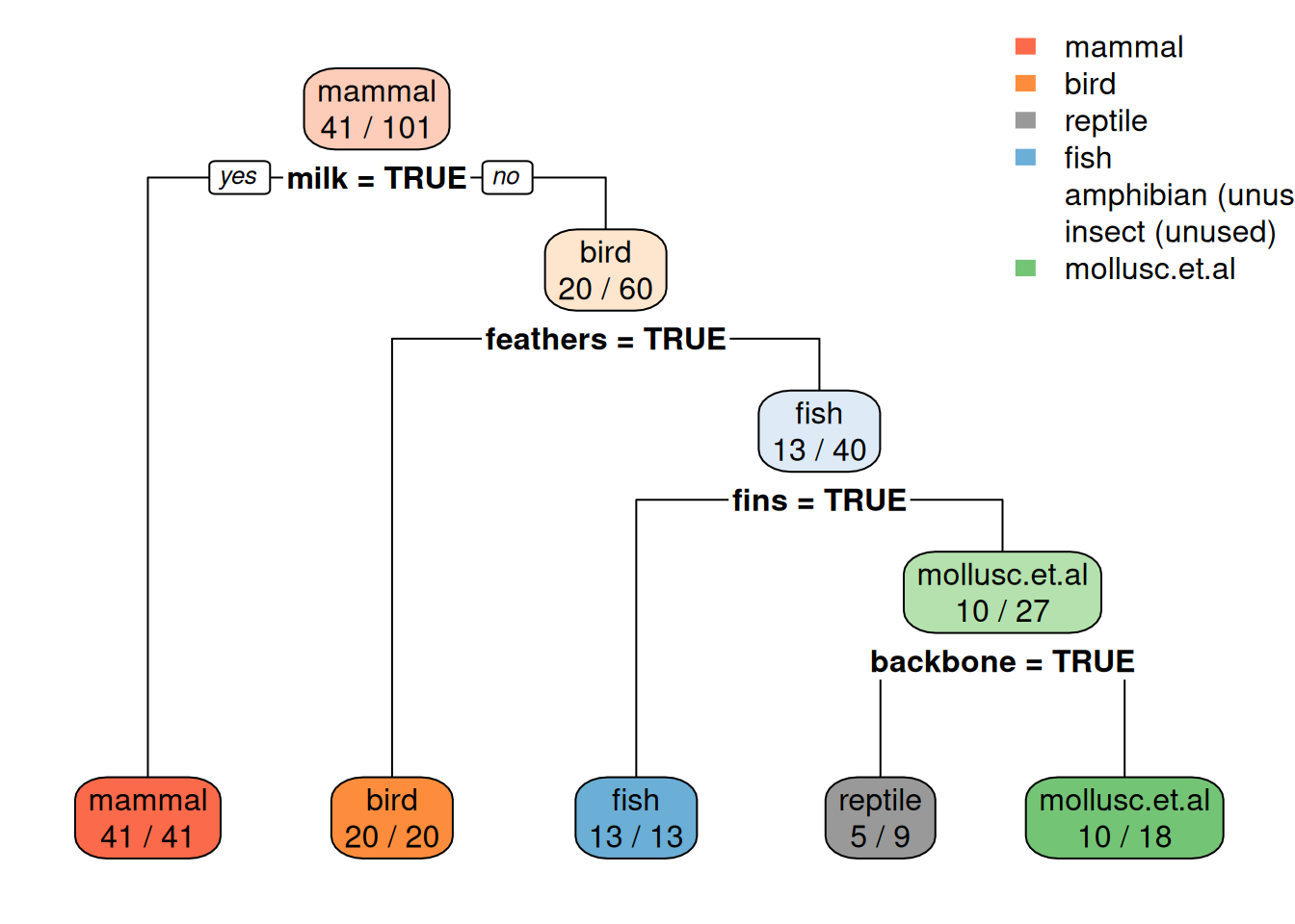
Note: extra=2 prints for each leaf node the number of correctly
classified objects from data and the total number of objects from the
training data falling into that node (correct/total).
3.5.2 Make Predictions for New Data
I will make up my own animal: A lion with feathered wings.
my_animal <- tibble(hair = TRUE, feathers = TRUE, eggs = FALSE,
  milk = TRUE, airborne = TRUE, aquatic = FALSE, predator = TRUE,
  toothed = TRUE, backbone = TRUE, breathes = TRUE,
  venomous = FALSE, fins = FALSE, legs = 4, tail = TRUE,
  domestic = FALSE, catsize = FALSE, type = NA)
The data types need to match the original data so we change the columns to be factors like in the training set.
my_animal <- my_animal |>
  mutate(across(where(is.logical),
                function(x) factor(x, levels = c(TRUE, FALSE))))
my_animal
## # A tibble: 1 × 17
##   hair  feathers eggs  milk  airborne aquatic predator
##   <fct> <fct>    <fct> <fct> <fct>    <fct>   <fct>
## 1 TRUE  TRUE     FALSE TRUE  TRUE     FALSE   TRUE
## # ℹ 10 more variables: toothed <fct>, backbone <fct>,
## #   breathes <fct>, venomous <fct>, fins <fct>, legs <dbl>,
## #   tail <fct>, domestic <fct>, catsize <fct>, type <fct>
Next, we make a prediction using the default tree
predict(tree_default , my_animal, type = "class")
##      1
## mammal
## 7 Levels: mammal bird reptile fish amphibian ... mollusc.et.al
3.5.3 Calculation of the Resubstitution Error
We will calculate error of the model on the training data manually first, so we see how it is calculated. The over all error (i.e., number of incorrectly classified examples) can be broken down into the error for each class. This information is typically presented in the form of a confusion matrix.
predict(tree_default, Zoo) |> head ()
##   mammal bird reptile fish amphibian insect mollusc.et.al
## 1      1    0       0    0         0      0             0
## 2      1    0       0    0         0      0             0
## 3      0    0       0    1         0      0             0
## 4      1    0       0    0         0      0             0
## 5      1    0       0    0         0      0             0
## 6      1    0       0    0         0      0             0
pred <- predict(tree_default, Zoo, type="class")
head(pred)
##      1      2      3      4      5      6
## mammal mammal   fish mammal mammal mammal
## 7 Levels: mammal bird reptile fish amphibian ... mollusc.et.al
We can easily tabulate the true and predicted labels to create a confusion matrix.
confusion_table <- with(Zoo, table(type, pred))
confusion_table
##                pred
## type            mammal bird reptile fish amphibian insect
##   mammal            41    0       0    0         0      0
##   bird               0   20       0    0         0      0
##   reptile            0    0       5    0         0      0
##   fish               0    0       0   13         0      0
##   amphibian          0    0       4    0         0      0
##   insect             0    0       0    0         0      0
##   mollusc.et.al      0    0       0    0         0      0
##                pred
## type            mollusc.et.al
##   mammal                    0
##   bird                      0
##   reptile                   0
##   fish                      0
##   amphibian                 0
##   insect                    8
##   mollusc.et.al            10
The counts in the diagonal are correct predictions. Off-diagonal counts represent errors (i.e., confusions).
We can summarize the confusion matrix using the accuracy measure.
correct <- confusion_table |> diag() |> sum()
correct
## [1] 89
error <- confusion_table |> sum() - correct
error
## [1] 12
Accuracy is just 1 \(-\) error rate and give the proportion of correctly classified examples.
accuracy <- correct / (correct + error)
accuracy
## [1] 0.8812
Here is the accuracy calculation as a simple function.
accuracy <- function(prediction, truth) {
    tbl <- table(truth, prediction)
    sum(diag(tbl))/sum(tbl)
}

accuracy(pred, Zoo |> pull(type))
## [1] 0.8812
The caret package provides a convenient way to calculate and analyze classification errors with the confusion matrix. It only needs the predicted class labels and the correct class labels as the reference.
library(caret)
## Loading required package: lattice
##
## Attaching package: 'caret'
## The following object is masked from 'package:purrr':
##
##     lift
confusionMatrix(data = pred,
                reference = Zoo |> pull(type))
## Confusion Matrix and Statistics
##
##                Reference
## Prediction      mammal bird reptile fish amphibian insect
##   mammal            41    0       0    0         0      0
##   bird               0   20       0    0         0      0
##   reptile            0    0       5    0         4      0
##   fish               0    0       0   13         0      0
##   amphibian          0    0       0    0         0      0
##   insect             0    0       0    0         0      0
##   mollusc.et.al      0    0       0    0         0      8
##                Reference
## Prediction      mollusc.et.al
##   mammal                    0
##   bird                      0
##   reptile                   0
##   fish                      0
##   amphibian                 0
##   insect                    0
##   mollusc.et.al            10
##
## Overall Statistics
##
##                Accuracy : 0.881
##                  95% CI : (0.802, 0.937)
##     No Information Rate : 0.406
##     P-Value [Acc > NIR] : <2e-16
##
##                   Kappa : 0.843
##
##  Mcnemar's Test P-Value : NA
##
## Statistics by Class:
##
##                      Class: mammal Class: bird
## Sensitivity                  1.000       1.000
## Specificity                  1.000       1.000
## Pos Pred Value               1.000       1.000
## Neg Pred Value               1.000       1.000
## Prevalence                   0.406       0.198
## Detection Rate               0.406       0.198
## Detection Prevalence         0.406       0.198
## Balanced Accuracy            1.000       1.000
##                      Class: reptile Class: fish
## Sensitivity                  1.0000       1.000
## Specificity                  0.9583       1.000
## Pos Pred Value               0.5556       1.000
## Neg Pred Value               1.0000       1.000
## Prevalence                   0.0495       0.129
## Detection Rate               0.0495       0.129
## Detection Prevalence         0.0891       0.129
## Balanced Accuracy            0.9792       1.000
##                      Class: amphibian Class: insect
## Sensitivity                    0.0000        0.0000
## Specificity                    1.0000        1.0000
## Pos Pred Value                    NaN           NaN
## Neg Pred Value                 0.9604        0.9208
## Prevalence                     0.0396        0.0792
## Detection Rate                 0.0000        0.0000
## Detection Prevalence           0.0000        0.0000
## Balanced Accuracy              0.5000        0.5000
##                      Class: mollusc.et.al
## Sensitivity                         1.000
## Specificity                         0.912
## Pos Pred Value                      0.556
## Neg Pred Value                      1.000
## Prevalence                          0.099
## Detection Rate                      0.099
## Detection Prevalence                0.178
## Balanced Accuracy                   0.956
In addition to the confusion matrix, it also includes additional statistics and measures. Details can be found in the Model Evaluation section.
Important note: Calculating accuracy on the training data is not a good idea! A complete example with code for holding out a test set and performing hyperparameter selection using cross-validation can be found in section Hyperparameter Tuning.
3.6 Model Overfitting
We are tempted to create the largest possible tree
to get the most accurate model. This can be achieved by
changing the algorithm’s hyperparameters (settings that
change how the algorithm works). We
set the complexity parameter cp to 0 (split
even if it does not improve the fit) and we set the minimum number of
observations in a node needed to split to the smallest value of 2 (see:
?rpart.control). Note: This is not a good idea!
As we will see later, full trees overfit the training data!
tree_full <- Zoo |>
  rpart(type ~ . , data = _,
        control = rpart.control(minsplit = 2, cp = 0))
rpart.plot(tree_full, extra = 2,
           roundint=FALSE,
           box.palette = list("Gy", "Gn", "Bu", "Bn",
"Or", "Rd", "Pu")) 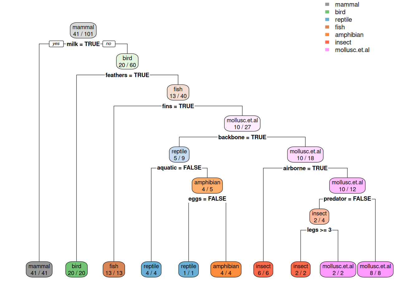
tree_full
## n= 101
##
## node), split, n, loss, yval, (yprob)
##       * denotes terminal node
##
##   1) root 101 60 mammal (0.41 0.2 0.05 0.13 0.04 0.079 0.099)
##     2) milk=TRUE 41  0 mammal (1 0 0 0 0 0 0) *
##     3) milk=FALSE 60 40 bird (0 0.33 0.083 0.22 0.067 0.13 0.17)
##       6) feathers=TRUE 20  0 bird (0 1 0 0 0 0 0) *
##       7) feathers=FALSE 40 27 fish (0 0 0.12 0.33 0.1 0.2 0.25)
##        14) fins=TRUE 13  0 fish (0 0 0 1 0 0 0) *
##        15) fins=FALSE 27 17 mollusc.et.al (0 0 0.19 0 0.15 0.3 0.37)
##          30) backbone=TRUE 9  4 reptile (0 0 0.56 0 0.44 0 0)
##            60) aquatic=FALSE 4  0 reptile (0 0 1 0 0 0 0) *
##            61) aquatic=TRUE 5  1 amphibian (0 0 0.2 0 0.8 0 0)
##             122) eggs=FALSE 1  0 reptile (0 0 1 0 0 0 0) *
##             123) eggs=TRUE 4  0 amphibian (0 0 0 0 1 0 0) *
##          31) backbone=FALSE 18  8 mollusc.et.al (0 0 0 0 0 0.44 0.56)
##            62) airborne=TRUE 6  0 insect (0 0 0 0 0 1 0) *
##            63) airborne=FALSE 12  2 mollusc.et.al (0 0 0 0 0 0.17 0.83)
##             126) predator=FALSE 4  2 insect (0 0 0 0 0 0.5 0.5)
##               252) legs>=3 2  0 insect (0 0 0 0 0 1 0) *
##               253) legs< 3 2  0 mollusc.et.al (0 0 0 0 0 0 1) *
##             127) predator=TRUE 8  0 mollusc.et.al (0 0 0 0 0 0 1) *
Error on the training set of the full tree
pred_full <- predict(tree_full, Zoo, type = "class")

accuracy(pred_full, Zoo |> pull(type))
## [1] 1
The training error is lower than that of the pruned tree. This, however, does not mean that the model is better. It actually is overfitting the training data (it just memorizes it) and it likely has worse generalization performance on new data. This effect is called overfitting the training data and needs to be avoided.
3.7 Model Selection
We often can create many different models for a classification problem. Above, we have created a decision tree using the default settings and also a full tree. The question is which model to use. This is called model selection.
In order to select the model we need to split the training data into a validation set and the training set that is actually used to train model. The error rate on the validation set can then be used to choose between several models.
caret supports model selection through its train() function. We will compare two trees
one with the default complexity cp = 0.01 and a full tree cp = 0. The values are set via tuneGrid.
trControl specified how the validation set is obtained. We use
Leave Group Out Cross-Validation (LGOCV) which
picks randomly a proportion p of data to train and uses the rest as
the validation set. To get a better estimate of the
error, this process is repeated number of times and the errors are averaged.
fit <- Zoo |>
  train(type ~ .,
    data = _ ,
    method = "rpart",
    control = rpart.control(minsplit = 2), # we have little data
    tuneGrid = data.frame(cp = c(0.01, 0)),
    trControl = trainControl(method = "LGOCV",
                             p = 0.8,
                             number = 10),
    tuneLength = 5)

fit
## CART
##
## 101 samples
##  16 predictor
##   7 classes: 'mammal', 'bird', 'reptile', 'fish', 'amphibian', 'insect', 'mollusc.et.al'
##
## No pre-processing
## Resampling: Repeated Train/Test Splits Estimated (10 reps, 80%)
## Summary of sample sizes: 83, 83, 83, 83, 83, 83, ...
## Resampling results across tuning parameters:
##
##   cp    Accuracy  Kappa
##   0.00  0.9722    0.9616
##   0.01  0.9667    0.9538
##
## Accuracy was used to select the optimal model using
##  the largest value.
## The final value used for the model was cp = 0.
We see that in this case, the full tree model performs slightly better. However, given the small dataset of 101 animals and the tiny validation set (20% of the animals), this may not be a significant difference and we will look at a statistical test for this later.
3.8 Model Evaluation
Models should be evaluated on a test set that has no overlap with the training set. We typically split the data using random sampling. To get reproducible results, we set random number generator seed.
set.seed(2000)3.8.1 Holdout Method
Test data is not used in the model building process and set aside purely for testing the model. Here, we partition data the 80% training and 20% testing.
inTrain <- createDataPartition(y = Zoo$type, p = .8)[[1]]
Zoo_train <- Zoo |> slice(inTrain)
Zoo_test <- Zoo |> slice(-inTrain)
Now we can train on the Zoo_train set and get the generalization error on the
Zoo_test set.
3.8.2 Cross-Validation Methods
There are several cross-validation methods that can use the available data more efficiently than the holdout method. The most popular method is k-fold cross-validation which splits the data randomly into \(k\) folds. It then holds one fold back for testing and trains on the other \(k-1\) folds. This is done with each fold and the resulting statistic (e.g., accuracy) is averaged. This method uses the data more efficiently than the holdout method.
Cross-validation can be used in train() with
trControl = trainControl(method = "cv", number = 10).
Cross-validation estimates predictive performance when the analysis is
specified in advance. If the same cross-validation results are used to choose
among many models, that estimate can be optimistic; use nested resampling or a
separate test set for a final assessment.
Cross-validation runs are independent and can be done faster in
parallel. To enable multi-core support, caret uses the package
foreach and you need to load a do backend. For Linux, you can use
doMC with 4 cores. Windows needs different backend like doParallel
(see the caret documentation).
## Linux backend
# library(doMC)
# registerDoMC(cores = 4)
# getDoParWorkers()

## Windows backend
# library(doParallel)
# cl <- makeCluster(4, type="SOCK")
# registerDoParallel(cl)
3.9 Hyperparameter Tuning
Note: This section contains a complete code example of how data should be used. It first holds out a test set and then performs hyperparameter selection using cross-validation.
Hyperparameters are parameters that change how a
training algorithm works. An example is the complexity parameter
cp for rpart decision trees. Tuning the hyperparameter means that
we want to perform model selection to pick the best setting.
We typically first use the holdout method to create a test set and then use cross validation using the training data for model selection. Let us use 80% for training and hold out 20% for testing.
inTrain <- createDataPartition(y = Zoo$type, p = .8)[[1]]
Zoo_train <- Zoo |> slice(inTrain)
Zoo_test <- Zoo |> slice(-inTrain)
The package caret combines training and validation for hyperparameter
tuning into the train() function. It internally splits the
data into training and validation sets and thus will provide you with
error estimates for different hyperparameter settings. trainControl is
used to choose how testing is performed.
For rpart, train tries to tune the cp parameter (tree complexity)
using accuracy to chose the best model. I set minsplit to 2 since we
have not much data. Note: Parameters used for tuning (in this case
cp) need to be set using a data.frame in the argument tuneGrid!
Setting it in control will be ignored.
fit <- Zoo_train |>
  train(type ~ .,
    data = _ ,
    method = "rpart",
    control = rpart.control(minsplit = 2), # we have little data
    trControl = trainControl(method = "cv", number = 10),
    tuneLength = 5)

fit
## CART
##
## 83 samples
## 16 predictors
##  7 classes: 'mammal', 'bird', 'reptile', 'fish', 'amphibian', 'insect', 'mollusc.et.al'
##
## No pre-processing
## Resampling: Cross-Validated (10 fold)
## Summary of sample sizes: 74, 73, 77, 75, 73, 75, ...
## Resampling results across tuning parameters:
##
##   cp    Accuracy  Kappa
##   0.00  0.9289    0.9058
##   0.08  0.8603    0.8179
##   0.16  0.7296    0.6422
##   0.22  0.6644    0.5448
##   0.32  0.4383    0.1136
##
## Accuracy was used to select the optimal model using
##  the largest value.
## The final value used for the model was cp = 0.
Note: Train has built 10 trees using the training folds for each
value of cp and the reported values for accuracy and Kappa are the
averages on the validation folds.
A model using the best tuning parameters and using all the data supplied
to train() is available as fit$finalModel.
library(rpart.plot)
rpart.plot(fit$finalModel, extra = 2,
  box.palette = list("Gy", "Gn", "Bu", "Bn", "Or", "Rd", "Pu"))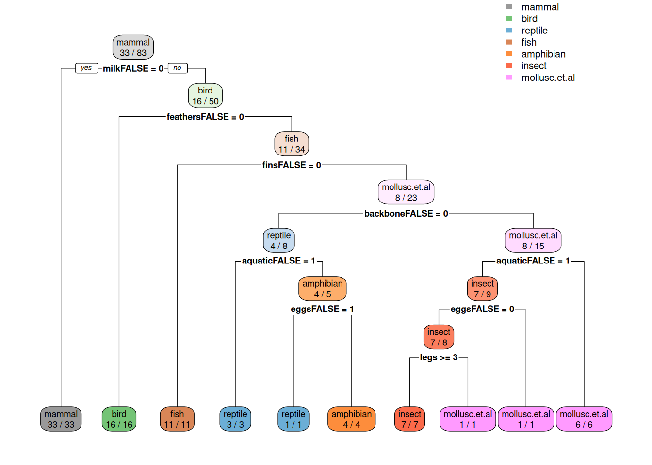
caret also computes variable importance. By default it uses competing
splits (splits which would be runners up, but do not get chosen by the
tree) for rpart models (see ? varImp). Toothed is the runner up for
many splits, but it never gets chosen!
varImp(fit)
## rpart variable importance
##
##               Overall
## toothedFALSE    100.0
## feathersFALSE    79.5
## eggsFALSE        67.7
## milkFALSE        63.3
## backboneFALSE    57.3
## finsFALSE        53.5
## hairFALSE        52.1
## breathesFALSE    48.9
## legs             41.4
## tailFALSE        29.0
## aquaticFALSE     27.5
## airborneFALSE    26.5
## predatorFALSE    10.6
## venomousFALSE     1.8
## catsizeFALSE      0.0
## domesticFALSE     0.0
Here is the variable importance without competing splits.
imp <- varImp(fit, compete = FALSE)
imp
## rpart variable importance
##
##               Overall
## milkFALSE      100.00
## feathersFALSE   55.69
## finsFALSE       39.45
## aquaticFALSE    28.11
## backboneFALSE   21.76
## eggsFALSE       12.32
## legs             7.28
## tailFALSE        0.00
## domesticFALSE    0.00
## airborneFALSE    0.00
## catsizeFALSE     0.00
## toothedFALSE     0.00
## venomousFALSE    0.00
## hairFALSE        0.00
## breathesFALSE    0.00
## predatorFALSE    0.00
ggplot(imp)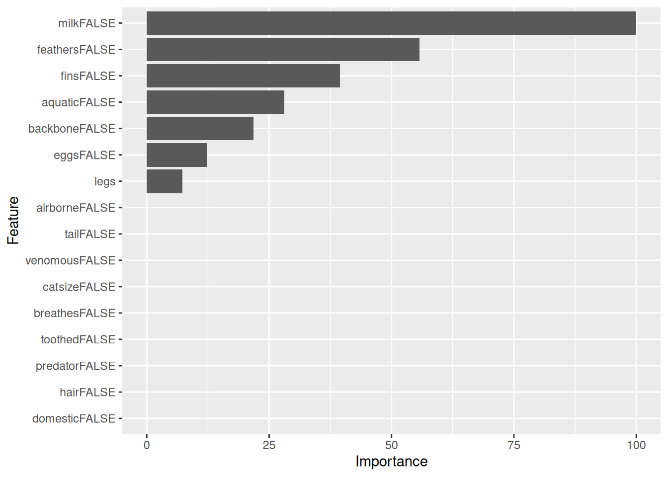
Note: Not all models provide a variable importance function. In this
case caret might calculate the variable importance by itself and ignore
the model (see ? varImp)!
Now, we can estimate the generalization error of the best model on the held out test data.
pred <- predict(fit, newdata = Zoo_test)
pred
##  [1] mammal        bird          mollusc.et.al bird
##  [5] mammal        mammal        insect        bird
##  [9] mammal        mammal        mammal        mammal
## [13] bird          fish          fish          reptile
## [17] mammal        mollusc.et.al
## 7 Levels: mammal bird reptile fish amphibian ... mollusc.et.al
Caret’s confusionMatrix() function calculates accuracy, confidence
intervals, kappa and many more evaluation metrics. You need to use
separate test data to create a confusion matrix based on the
generalization error.
confusionMatrix(data = pred,
                ref = Zoo_test |> pull(type))
## Confusion Matrix and Statistics
##
##                Reference
## Prediction      mammal bird reptile fish amphibian insect
##   mammal             8    0       0    0         0      0
##   bird               0    4       0    0         0      0
##   reptile            0    0       1    0         0      0
##   fish               0    0       0    2         0      0
##   amphibian          0    0       0    0         0      0
##   insect             0    0       0    0         0      1
##   mollusc.et.al      0    0       0    0         0      0
##                Reference
## Prediction      mollusc.et.al
##   mammal                    0
##   bird                      0
##   reptile                   0
##   fish                      0
##   amphibian                 0
##   insect                    0
##   mollusc.et.al             2
##
## Overall Statistics
##
##                Accuracy : 1
##                  95% CI : (0.815, 1)
##     No Information Rate : 0.444
##     P-Value [Acc > NIR] : 4.58e-07
##
##                   Kappa : 1
##
##  Mcnemar's Test P-Value : NA
##
## Statistics by Class:
##
##                      Class: mammal Class: bird
## Sensitivity                  1.000       1.000
## Specificity                  1.000       1.000
## Pos Pred Value               1.000       1.000
## Neg Pred Value               1.000       1.000
## Prevalence                   0.444       0.222
## Detection Rate               0.444       0.222
## Detection Prevalence         0.444       0.222
## Balanced Accuracy            1.000       1.000
##                      Class: reptile Class: fish
## Sensitivity                  1.0000       1.000
## Specificity                  1.0000       1.000
## Pos Pred Value               1.0000       1.000
## Neg Pred Value               1.0000       1.000
## Prevalence                   0.0556       0.111
## Detection Rate               0.0556       0.111
## Detection Prevalence         0.0556       0.111
## Balanced Accuracy            1.0000       1.000
##                      Class: amphibian Class: insect
## Sensitivity                        NA        1.0000
## Specificity                         1        1.0000
## Pos Pred Value                     NA        1.0000
## Neg Pred Value                     NA        1.0000
## Prevalence                          0        0.0556
## Detection Rate                      0        0.0556
## Detection Prevalence                0        0.0556
## Balanced Accuracy                  NA        1.0000
##                      Class: mollusc.et.al
## Sensitivity                         1.000
## Specificity                         1.000
## Pos Pred Value                      1.000
## Neg Pred Value                      1.000
## Prevalence                          0.111
## Detection Rate                      0.111
## Detection Prevalence                0.111
## Balanced Accuracy                   1.000
Definitions of the additional statistics by class (including alternative names) can be found in caret’s confusion matrix man page.
Some notes
- Many classification algorithms and
trainin caret do not deal well with missing values. If your classification model can deal with missing values (e.g.,rpart) then usena.action = na.passwhen you calltrainandpredict. Otherwise, you need to remove observations with missing values withna.omitor use imputation to replace the missing values before you train the model. Make sure that you still have enough observations left. - Make sure that nominal variables (this includes logical variables) are coded as factors.
- The class variable for train in caret cannot have level names that
are keywords in R (e.g.,
TRUEandFALSE). Rename them to, for example, “yes” and “no.” - Make sure that nominal variables (factors) have examples for all
possible values. Some methods might have problems with variable
values without examples. You can drop empty levels using
droplevelsorfactor. - Sampling in train might create a sample that does not contain examples for all values in a nominal (factor) variable. You will get an error message. This most likely happens for variables which have one very rare value. You may have to remove the variable.
3.10 Pitfalls of Model Selection and Evaluation
- Do not use training error as an estimate of performance on new data. If you select a model using validation results, those results are not an independent final assessment. Reserve a test set or use nested resampling for that purpose.
- The training data and test data must not overlap, or the evaluation will not measure performance on new data. Leakage can also occur if preprocessing or feature selection uses the full dataset before the split.
3.11 Model Comparison
We will compare three models: a majority-class baseline, a decision tree, and
a k-nearest neighbors (kNN) classifier. We will use 10-fold cross-validation
for hyperparameter tuning.
caret::train() selects tuning settings from the resampling results and fits a
final model using all supplied training data. The resampling results estimate
performance and support model comparison, but do not by themselves establish
that one model is significantly better.
3.11.1 Build models
caret does not provide a baseline classifier, but the package basemodels does.
We first create a simple baseline model that always predicts the majority
class mammal.
baseline <- Zoo_train |> train(type ~ .,
  method = basemodels::dummyClassifier,
  data = _,
  strategy = "constant",
  constant = "mammal",
  trControl = trainControl(method = "cv"
                           ))
baseline
## dummyClassifier
##
## 83 samples
## 16 predictors
##  7 classes: 'mammal', 'bird', 'reptile', 'fish', 'amphibian', 'insect', 'mollusc.et.al'
##
## No pre-processing
## Resampling: Cross-Validated (10 fold)
## Summary of sample sizes: 73, 74, 73, 75, 74, 77, ...
## Resampling results:
##
##   Accuracy  Kappa
##   0.4047    0
The second model is a default decision tree.
rpartFit <- Zoo_train |>
  train(type ~ .,
        data = _,
        method = "rpart",
        tuneLength = 10,
        trControl = trainControl(method = "cv")
  )
rpartFit
## CART
##
## 83 samples
## 16 predictors
##  7 classes: 'mammal', 'bird', 'reptile', 'fish', 'amphibian', 'insect', 'mollusc.et.al'
##
## No pre-processing
## Resampling: Cross-Validated (10 fold)
## Summary of sample sizes: 75, 75, 75, 73, 76, 72, ...
## Resampling results across tuning parameters:
##
##   cp       Accuracy  Kappa
##   0.00000  0.7841    0.7195
##   0.03556  0.7841    0.7195
##   0.07111  0.7841    0.7195
##   0.10667  0.7841    0.7182
##   0.14222  0.7841    0.7182
##   0.17778  0.7271    0.6369
##   0.21333  0.7071    0.6109
##   0.24889  0.5940    0.4423
##   0.28444  0.5940    0.4423
##   0.32000  0.4968    0.2356
##
## Accuracy was used to select the optimal model using
##  the largest value.
## The final value used for the model was cp = 0.1422.
The third model is a kNN classifier, this classifier will be discussed
in the next Chapter. kNN uses the Euclidean distance between objects.
Logicals will be used as 0-1 variables. To make sure the range of all
variables is compatible, we
ask train to scale the data using
preProcess = "scale".
knnFit <- Zoo_train |>
  train(type ~ .,
        data = _,
        method = "knn",
        preProcess = "scale",
          tuneLength = 10,
          trControl = trainControl(method = "cv")
  )
knnFit
## k-Nearest Neighbors
##
## 83 samples
## 16 predictors
##  7 classes: 'mammal', 'bird', 'reptile', 'fish', 'amphibian', 'insect', 'mollusc.et.al'
##
## Pre-processing: scaled (16)
## Resampling: Cross-Validated (10 fold)
## Summary of sample sizes: 75, 74, 74, 74, 74, 75, ...
## Resampling results across tuning parameters:
##
##   k   Accuracy  Kappa
##    5  0.9092    0.8835
##    7  0.8715    0.8301
##    9  0.8579    0.8113
##   11  0.8590    0.8131
##   13  0.8727    0.8302
##   15  0.8727    0.8302
##   17  0.8490    0.7989
##   19  0.8490    0.7967
##   21  0.7943    0.7219
##   23  0.7943    0.7217
##
## Accuracy was used to select the optimal model using
##  the largest value.
## The final value used for the model was k = 5.
Compare the accuracy and kappa distributions of the final model over all folds.
resamps <- resamples(list(
    baseline = baseline,
  CART = rpartFit,
        kNearestNeighbors = knnFit
        ))

summary(resamps)
##
## Call:
## summary.resamples(object = resamps)
##
## Models: baseline, CART, kNearestNeighbors
## Number of resamples: 10
##
## Accuracy
##                     Min. 1st Qu. Median   Mean 3rd Qu.
## baseline          0.3000   0.375 0.3875 0.4047  0.4444
## CART              0.7143   0.733 0.7639 0.7841  0.8429
## kNearestNeighbors 0.7778   0.875 0.8819 0.9092  1.0000
##                    Max. NA's
## baseline          0.500    0
## CART              0.875    0
## kNearestNeighbors 1.000    0
##
## Kappa
##                     Min. 1st Qu. Median   Mean 3rd Qu.
## baseline          0.0000  0.0000 0.0000 0.0000  0.0000
## CART              0.6316  0.6622 0.6994 0.7182  0.7917
## kNearestNeighbors 0.7188  0.8307 0.8486 0.8835  1.0000
##                    Max. NA's
## baseline          0.000    0
## CART              0.814    0
## kNearestNeighbors 1.000    0
caret provides some visualizations. For
example, a boxplot to compare the accuracy and kappa distribution (over
the 10 folds).
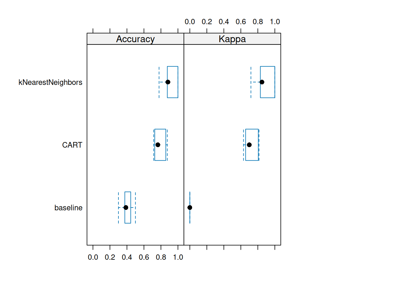
The baseline has no predictive power and consistently produces a kappa of 0.
KNN has the highest accuracy and kappa in these resampling results.
diff() reports paired comparisons of resampling results, including adjusted
p-values. Resampling folds are not independent observations, so treat these
tests as exploratory rather than definitive evidence that one model is better.
difs <- diff(resamps)
difs
##
## Call:
## diff.resamples(x = resamps)
##
## Models: baseline, CART, kNearestNeighbors
## Metrics: Accuracy, Kappa
## Number of differences: 3
## p-value adjustment: bonferroni
summary(difs)
##
## Call:
## summary.diff.resamples(object = difs)
##
## p-value adjustment: bonferroni
## Upper diagonal: estimates of the difference
## Lower diagonal: p-value for H0: difference = 0
##
## Accuracy
##                   baseline CART   kNearestNeighbors
## baseline                   -0.379 -0.504
## CART              5.19e-06        -0.125
## kNearestNeighbors 4.03e-08 0.031
##
## Kappa
##                   baseline CART   kNearestNeighbors
## baseline                   -0.718 -0.884
## CART              5.79e-10        -0.165
## kNearestNeighbors 2.87e-09 0.0206
The p-values quantify compatibility with a zero mean difference under the
test’s assumptions; they are not the probability that the null hypothesis is
true. diff() applies a Bonferroni adjustment for multiple comparisons. In
this small example, inspect the estimated differences and their uncertainty,
and use an independent test set for the final performance assessment.
3.12 Feature Selection*
Decision trees implicitly select features for splitting, but we can also select features before we apply any learning algorithm. Since different features lead to different models, choosing the best set of features is also a type of model selection.
Many feature selection methods are implemented in the FSelector package.
3.12.1 Univariate Feature Importance Score
These scores measure how related each feature is to the class variable. For discrete features (as in our case), the chi-square statistic can be used to derive a score.
weights <- Zoo_train |>
  chi.squared(type ~ ., data = _) |>
  as_tibble(rownames = "feature") |>
  arrange(desc(attr_importance))

weights
## # A tibble: 16 × 2
##    feature  attr_importance
##    <chr>              <dbl>
##  1 feathers           1
##  2 milk               1
##  3 backbone           1
##  4 toothed            0.981
##  5 eggs               0.959
##  6 breathes           0.917
##  7 hair               0.906
##  8 fins               0.845
##  9 legs               0.834
## 10 airborne           0.818
## 11 tail               0.779
## 12 aquatic            0.725
## 13 catsize            0.602
## 14 venomous           0.520
## 15 predator           0.374
## 16 domestic           0.256
We can plot the importance in descending order (using reorder to order factor
levels used by ggplot).
ggplot(weights,
  aes(x = attr_importance,
      y = reorder(feature, attr_importance))) +
  geom_bar(stat = "identity") +
  xlab("Importance score") +
  ylab("Feature")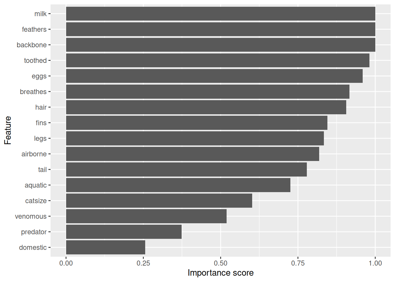
Picking the best features is called the feature ranking approach. Here we pick the 5 highest-ranked features.
subset <- cutoff.k(weights |>
                   column_to_rownames("feature"),
                   5)
subset
## [1] "feathers" "milk"     "backbone" "toothed"  "eggs"
Use only the selected features to build a model (Fselector provides
as.simple.formula).
f <- as.simple.formula(subset, "type")
f
## type ~ feathers + milk + backbone + toothed + eggs
## <environment: 0x559dc8cf81d0>
m <- Zoo_train |> rpart(f, data = _)
rpart.plot(m, extra = 2, roundint = FALSE)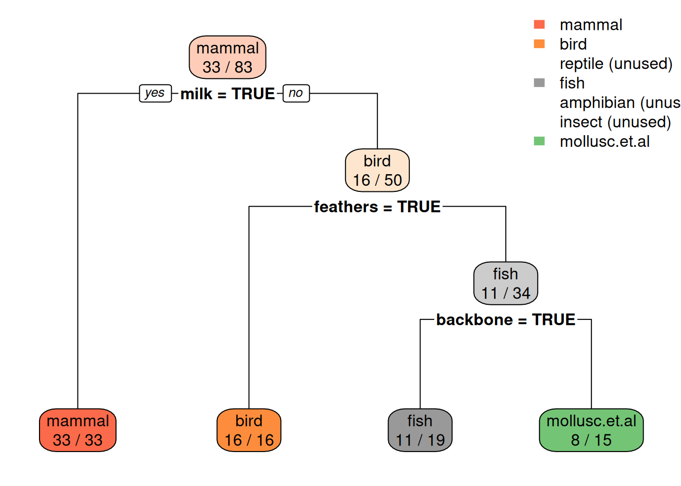
There are many alternative ways to calculate univariate importance scores (see package FSelector). Some of them (also) work for continuous features. One example is the information gain ratio based on entropy as used in decision tree induction.
Zoo_train |>
  gain.ratio(type ~ ., data = _) |>
  as_tibble(rownames = "feature") |>
  arrange(desc(attr_importance))
## # A tibble: 16 × 2
##    feature  attr_importance
##    <chr>              <dbl>
##  1 milk               1
##  2 backbone           1
##  3 feathers           1
##  4 toothed            0.959
##  5 eggs               0.907
##  6 breathes           0.845
##  7 hair               0.781
##  8 fins               0.689
##  9 legs               0.689
## 10 airborne           0.633
## 11 tail               0.573
## 12 aquatic            0.474
## 13 venomous           0.429
## 14 catsize            0.310
## 15 domestic           0.115
## 16 predator           0.110
3.12.2 Feature Subset Selection
Often, features are related and calculating importance for each feature
independently is not optimal. We can use greedy search heuristics. For
example cfs uses correlation/entropy with best first search.
Zoo_train |>
  cfs(type ~ ., data = _)
##  [1] "hair"     "feathers" "eggs"     "milk"     "toothed"
##  [6] "backbone" "breathes" "fins"     "legs"     "tail"
The disadvantage of this method is that the model we want to train may not use
correlation/entropy. We can use the actual model using
as a black-box defined in an evaluator function
to calculate a score to be maximized.
This is typically the best method, since it can use the model
for selection.
First, we define an evaluation
function that builds a model given a subset of features and calculates a
quality score. We use here the average for 5 bootstrap samples
(method = "cv" can also be used instead), no tuning (to be faster),
and the average accuracy as the score.
evaluator <- function(subset) {
  model <- Zoo_train |>
    train(as.simple.formula(subset, "type"),
          data = _,
          method = "rpart",
          trControl = trainControl(method = "boot", number = 5),
          tuneLength = 0)

  results <- model$resample$Accuracy

  cat("Trying features:", paste(subset, collapse = " + "), "\n")

  m <- mean(results)
  cat("Accuracy:", round(m, 2), "\n\n")
  m
}
Start with all features (but not the class variable type)
There are several (greedy) search strategies available. These run for a while so they commented out below. Remove the comment for one at a time to try these types of feature selection.
#subset <- backward.search(features, evaluator)
#subset <- forward.search(features, evaluator)
#subset <- best.first.search(features, evaluator)
#subset <- hill.climbing.search(features, evaluator)
#subset
3.13 Using Dummy Variables for Nominal Features*
Nominal features (factors) are often encoded as a series of 0-1 dummy variables. This approach is in machine learning often called one-hot encoding.
For example, let us try to predict if an animal is a predator given the type. First we use the original encoding of type as a factor with several values.
tree_predator <- Zoo_train |>
  rpart(predator ~ type, data = _)
rpart.plot(tree_predator, extra = 2, roundint = FALSE)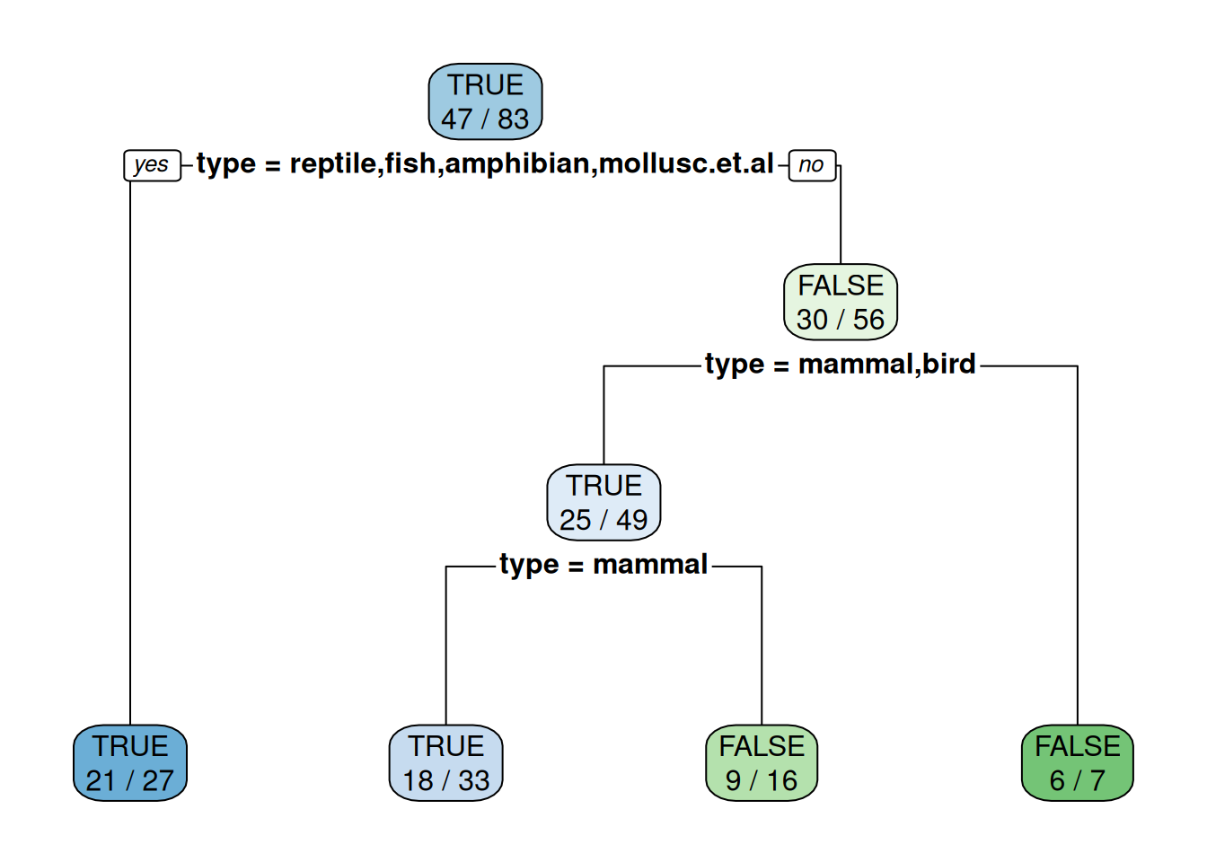
Note: Some splits use multiple values. Building the tree will become extremely slow if a factor has many levels (different values) since the tree has to check all possible splits into two subsets which has a time complexity of \(O(2^n)\) where \(n\) is the number of different values. This situation should be avoided.
We can convert the factor type into a set of 0-1 dummy variables using caret’s class2ind(). See
also ? dummyVars in package caret.
Zoo_train_dummy <- as_tibble(class2ind(Zoo_train$type)) |>
  mutate(across(everything(), as.factor)) |>
  add_column(predator = Zoo_train$predator)
Zoo_train_dummy
## # A tibble: 83 × 8
##    mammal bird  reptile fish  amphibian insect mollusc.et.al
##    <fct>  <fct> <fct>   <fct> <fct>     <fct>  <fct>
##  1 1      0     0       0     0         0      0
##  2 0      0     0       1     0         0      0
##  3 1      0     0       0     0         0      0
##  4 1      0     0       0     0         0      0
##  5 1      0     0       0     0         0      0
##  6 1      0     0       0     0         0      0
##  7 0      0     0       1     0         0      0
##  8 0      0     0       1     0         0      0
##  9 1      0     0       0     0         0      0
## 10 1      0     0       0     0         0      0
## # ℹ 73 more rows
## # ℹ 1 more variable: predator <fct>
tree_predator <- Zoo_train_dummy |>
  rpart(predator ~ .,
        data = _,
        control = rpart.control(minsplit = 2, cp = 0.01))
rpart.plot(tree_predator, roundint = FALSE)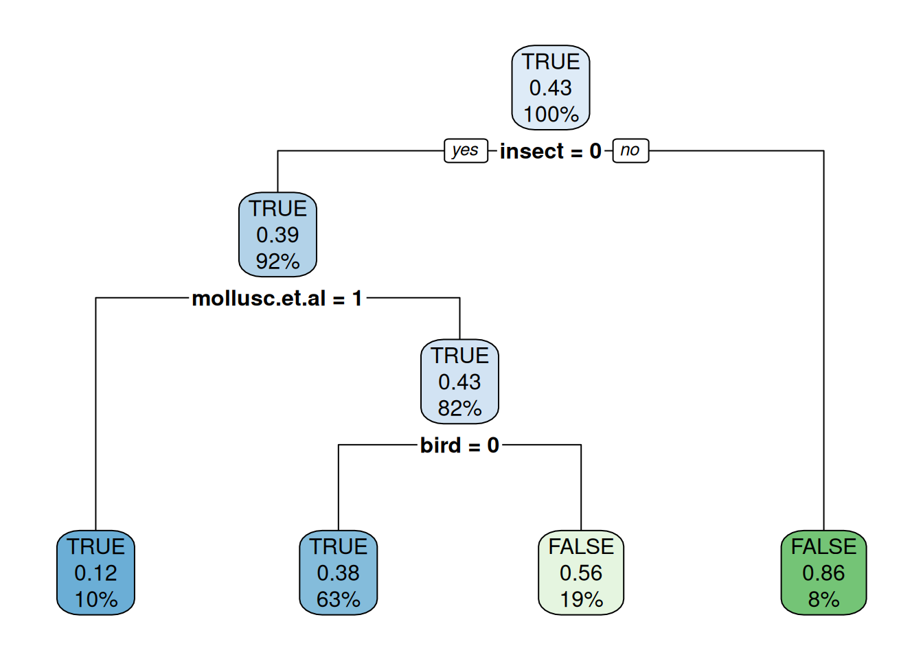
Using caret on the original factor encoding automatically translates
factors (here type) into 0-1 dummy variables (e.g., typeinsect = 0).
The reason is that some models cannot directly use factors and caret
tries to consistently work with all of them.
fit <- Zoo_train |>
  train(predator ~ type,
        data = _,
        method = "rpart",
        control = rpart.control(minsplit = 2),
        tuneGrid = data.frame(cp = 0.01))
fit
## CART
##
## 83 samples
##  1 predictor
##  2 classes: 'TRUE', 'FALSE'
##
## No pre-processing
## Resampling: Bootstrapped (25 reps)
## Summary of sample sizes: 83, 83, 83, 83, 83, 83, ...
## Resampling results:
##
##   Accuracy  Kappa
##   0.54      0.07527
##
## Tuning parameter 'cp' was held constant at a value of 0.01
rpart.plot(fit$finalModel, extra = 2)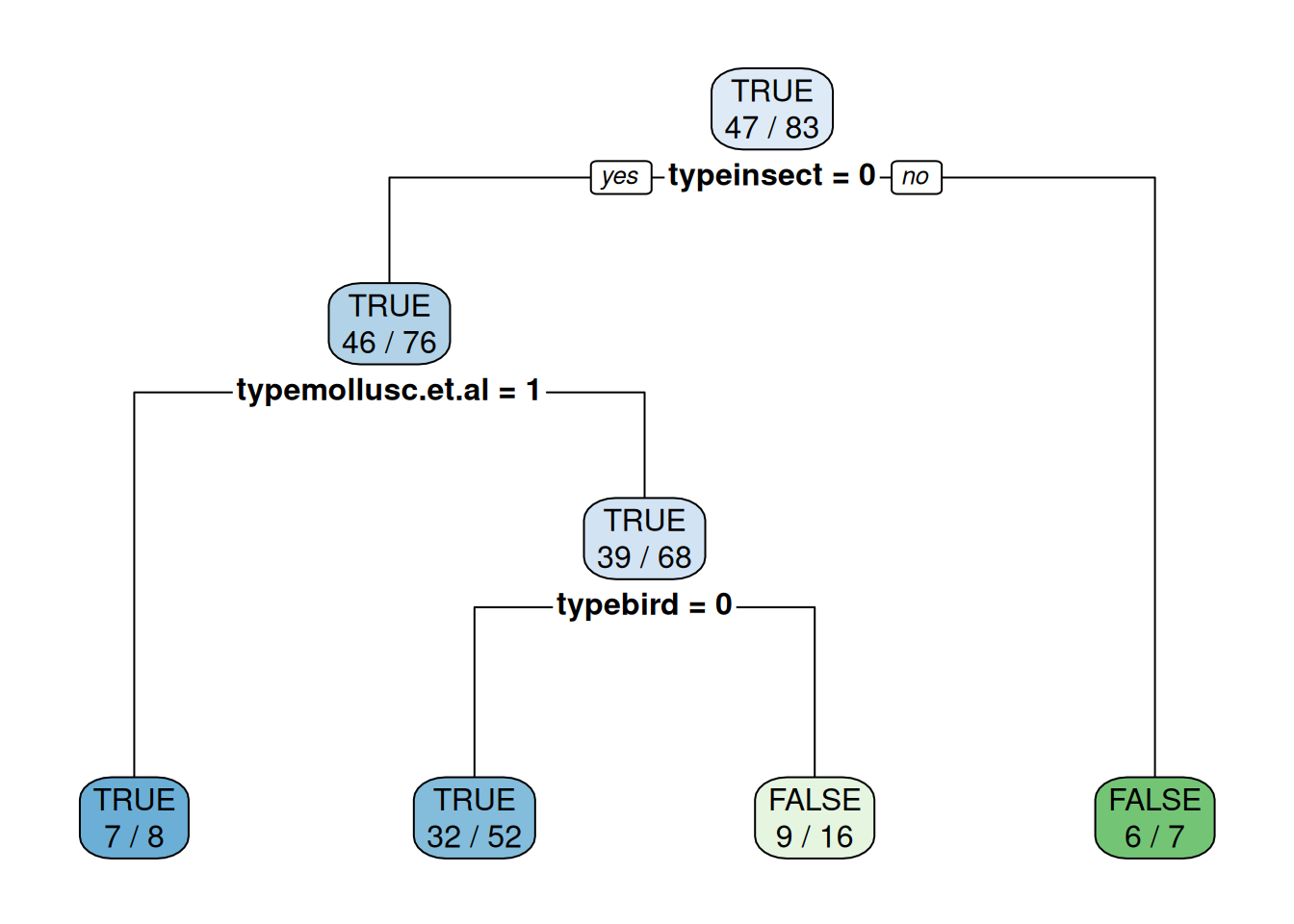
Note: To use a fixed value for the tuning parameter cp, we have to
create a tuning grid that only contains that value.
3.14 Exercises*
We will use again the Palmer penguin data for the exercises.
library(palmerpenguins)
##
## Attaching package: 'palmerpenguins'
## The following objects are masked from 'package:datasets':
##
##     penguins, penguins_raw
head(penguins)
## # A tibble: 6 × 8
##   species island    bill_length_mm bill_depth_mm
##   <fct>   <fct>              <dbl>         <dbl>
## 1 Adelie  Torgersen           39.1          18.7
## 2 Adelie  Torgersen           39.5          17.4
## 3 Adelie  Torgersen           40.3          18
## 4 Adelie  Torgersen           NA            NA
## 5 Adelie  Torgersen           36.7          19.3
## 6 Adelie  Torgersen           39.3          20.6
## # ℹ 4 more variables: flipper_length_mm <int>,
## #   body_mass_g <int>, sex <fct>, year <int>
Create a R markdown file with the code and discussion for the following below. Remember, the complete approach is described in section Hyperparameter Tuning.
- Split the data into a training and test set.
- Create an rpart decision tree to predict the species. You will have to deal with missing values.
- Experiment with setting
minsplitfor rpart and make suretuneLengthis at least 5. Discuss the model selection process (hyperparameter tuning) and what final model was chosen. - Visualize the tree and discuss what the splits mean.
- Calculate the variable importance from the fitted model. What variables are the most important? What variables do not matter?
- Use the test set to evaluate the generalization error and accuracy.
A good answer should describe the split and missing-value handling, and
show that tuning was done using training data only. Explain the selected
minsplit, the tree’s main splits, and what variable importance can and
cannot tell you. Report test-set results with enough detail to judge errors
across species, and distinguish this final evaluation from model selection.
3.15 Chapter Summary
Classification uses labeled examples to learn a mapping from input features to class labels. Decision trees provide an interpretable model, but a tree that fits its training data too closely may overfit. Separate data for fitting, model selection, and final evaluation; use holdout or cross-validation methods to estimate performance, tune hyperparameters without using the test set, and compare candidate models on consistent resamples. Choose evaluation measures that reflect the task and class distribution, and avoid leakage and other pitfalls in model selection. The chapter also introduces feature importance and subset selection, and dummy-variable encoding for nominal predictors.
3.16 Key Terms
- Classifier: a model that predicts a categorical class label.
- Resubstitution error: error measured on the same data used to fit a model.
- Cross-validation: repeated fitting and validation across data folds.
- Hyperparameter: a user-chosen setting that controls how a learning algorithm fits a model.
- Generalization error: expected prediction error on new, unseen data.