4 Classification: Alternative Techniques
This chapter introduces different types of classifiers. It also discusses the important problem of class imbalance in data and options to deal with it. In addition, this chapter compares visually the decision boundaries used by different algorithms. This will provide a better understanding of the model bias that different algorithms have.
4.1 Learning Objectives
After this chapter, you should be able to:
- describe the basic behavior of several common classification algorithms;
- compare models using a baseline and a consistent evaluation procedure;
- explain how class imbalance affects predictions and metrics; and
- compare decision boundaries and adjust a classifier’s decision threshold.
4.2 Prerequisites
Read Classification: Basic Concepts. Familiarity with model training, cross-validation, confusion matrices, and probability is assumed.
Packages Used in this Chapter
pkgs <- c("basemodels", "C50", "caret", "e1071", "klaR",
          "lattice", "MASS", "mlbench", "nnet", "palmerpenguins",
          "randomForest", "rpart", "RWeka", "scales", "tidyverse")

pak::pkg_install(pkgs)
The packages used for this chapter are:
- basemodels (Chen et al. 2023)
- C50 (Kuhn and Quinlan 2025)
- caret (Kuhn 2024)
- e1071 (Meyer et al. 2025)
- klaR (Roever et al. 2026)
- lattice (Sarkar 2026)
- MASS (B. Ripley and Venables 2026)
- mlbench (Leisch and Dimitriadou 2026)
- nnet (B. Ripley 2026)
- palmerpenguins (Horst, Hill, and Gorman 2022)
- randomForest (Breiman et al. 2024)
- rpart (Therneau and Atkinson 2026)
- RWeka (Hornik 2026)
- scales (Wickham, Pedersen, and Seidel 2025)
- tidyverse (Wickham 2023)
4.3 Types of Classifiers
Many different classification algorithms have been proposed in the literature. In this chapter, we will apply some of the more popular methods.
4.3.1 Set up the Training and Test Data
We will use the Zoo dataset which is included in the R package mlbench
(you may have to install it). The Zoo dataset containing 17 (mostly
logical) variables on different 101 animals as a data frame with 17
columns (hair, feathers, eggs, milk, airborne, aquatic, predator,
toothed, backbone, breathes, venomous, fins, legs, tail, domestic,
catsize, type). We convert the data frame into a tidyverse tibble
(optional).
library(tidyverse)
data(Zoo, package = "mlbench")

Zoo <- as_tibble(Zoo)
Zoo
## # A tibble: 101 × 17
##    hair  feathers eggs  milk  airborne aquatic predator
##    <lgl> <lgl>    <lgl> <lgl> <lgl>    <lgl>   <lgl>
##  1 TRUE  FALSE    FALSE TRUE  FALSE    FALSE   TRUE
##  2 TRUE  FALSE    FALSE TRUE  FALSE    FALSE   FALSE
##  3 FALSE FALSE    TRUE  FALSE FALSE    TRUE    TRUE
##  4 TRUE  FALSE    FALSE TRUE  FALSE    FALSE   TRUE
##  5 TRUE  FALSE    FALSE TRUE  FALSE    FALSE   TRUE
##  6 TRUE  FALSE    FALSE TRUE  FALSE    FALSE   FALSE
##  7 TRUE  FALSE    FALSE TRUE  FALSE    FALSE   FALSE
##  8 FALSE FALSE    TRUE  FALSE FALSE    TRUE    FALSE
##  9 FALSE FALSE    TRUE  FALSE FALSE    TRUE    TRUE
## 10 TRUE  FALSE    FALSE TRUE  FALSE    FALSE   FALSE
## # ℹ 91 more rows
## # ℹ 10 more variables: toothed <lgl>, backbone <lgl>,
## #   breathes <lgl>, venomous <lgl>, fins <lgl>, legs <int>,
## #   tail <lgl>, domestic <lgl>, catsize <lgl>, type <fct>
The examples use caret for data splitting,
model fitting, and tuning, while specialist packages provide the algorithms.
This book uses the caret interface; it does not implement the same examples
with tidymodels.
Multi-core support can be used for cross-validation. Note: It is commented out here because it does not work with rJava used by the RWeka-based classifiers below.
##library(doMC, quietly = TRUE)
##registerDoMC(cores = 4)
##getDoParWorkers()
Test data is not used in the model building process and needs to be set aside purely for testing the model after it is completely built. Here I use 80% for training.
inTrain <- createDataPartition(y = Zoo$type, p = .8)[[1]]
Zoo_train <- Zoo |> slice(inTrain)
Zoo_test <- Zoo |> slice(-inTrain)
For hyperparameter tuning, we will use 10-fold cross-validation.
Note: Be careful if you have many NA values in your data.
train() and cross-validation many fail in some cases. If that is the
case then you can remove features (columns) which have many NAs, omit
NAs using na.omit() or use imputation to replace them with
reasonable values (e.g., by the feature mean or via kNN). Highly
imbalanced datasets are also problematic since there is a chance that a
fold does not contain examples of each class leading to a hard to
understand error message.
4.4 Rule-based classifier: PART
rulesFit <- Zoo_train |> train(type ~ .,
  method = "PART",
  data = _,
  tuneLength = 5,
  trControl = trainControl(method = "cv"))
rulesFit
## Rule-Based Classifier
##
## 83 samples
## 16 predictors
##  7 classes: 'mammal', 'bird', 'reptile', 'fish', 'amphibian', 'insect', 'mollusc.et.al'
##
## No pre-processing
## Resampling: Cross-Validated (10 fold)
## Summary of sample sizes: 74, 74, 74, 74, 75, 75, ...
## Resampling results across tuning parameters:
##
##   threshold  pruned  Accuracy  Kappa
##   0.0100     yes     0.9542    0.9382
##   0.0100     no      0.9288    0.9060
##   0.1325     yes     0.9542    0.9382
##   0.1325     no      0.9288    0.9060
##   0.2550     yes     0.9542    0.9382
##   0.2550     no      0.9288    0.9060
##   0.3775     yes     0.9542    0.9382
##   0.3775     no      0.9288    0.9060
##   0.5000     yes     0.9542    0.9382
##   0.5000     no      0.9288    0.9060
##
## Accuracy was used to select the optimal model using
##  the largest value.
## The final values used for the model were threshold =
##  0.5 and pruned = yes.
The model selection results are shown in the table. This is the selected model:
rulesFit$finalModel
## PART decision list
## ------------------
##
## feathersTRUE <= 0 AND
## milkTRUE > 0: mammal (33.0)
##
## feathersTRUE > 0: bird (16.0)
##
## backboneTRUE <= 0 AND
## airborneTRUE <= 0: mollusc.et.al (9.0/1.0)
##
## airborneTRUE <= 0 AND
## finsTRUE > 0: fish (11.0)
##
## airborneTRUE > 0: insect (6.0)
##
## aquaticTRUE > 0: amphibian (5.0/1.0)
##
## : reptile (3.0)
##
## Number of Rules  :   7
PART returns a decision list, i.e., an ordered rule set. For example, the first rule shows that an animal with no feathers but milk is a mammal. I ordered rule sets, the decision of the first matching rule is used.
4.5 Nearest Neighbor Classifier
K-Nearest neighbor classifiers classify a new data point by looking at the
majority class labels of its k nearest neighbors in the training data set.
The used kNN implementation uses Euclidean distance to determine what data points
are near by, so data needs be standardized
(scaled) first. Here legs are measured between 0 and 6 while all other
variables are between 0 and 1. Scaling to z-scores can be directly performed as
preprocessing in train using the parameter preProcess = "scale".
The \(k\) value is typically choose as an odd number so we get a clear majority.
knnFit <- Zoo_train |> train(type ~ .,
  method = "knn",
  data = _,
  preProcess = "scale",
  tuneGrid = data.frame(k = c(1, 3, 5, 7, 9)),
    trControl = trainControl(method = "cv"))
knnFit
## k-Nearest Neighbors
##
## 83 samples
## 16 predictors
##  7 classes: 'mammal', 'bird', 'reptile', 'fish', 'amphibian', 'insect', 'mollusc.et.al'
##
## Pre-processing: scaled (16)
## Resampling: Cross-Validated (10 fold)
## Summary of sample sizes: 75, 73, 74, 75, 74, 74, ...
## Resampling results across tuning parameters:
##
##   k  Accuracy  Kappa
##   1  0.9428    0.9256
##   3  0.9410    0.9234
##   5  0.9299    0.9088
##   7  0.9031    0.8728
##   9  0.9031    0.8721
##
## Accuracy was used to select the optimal model using
##  the largest value.
## The final value used for the model was k = 1.
knnFit$finalModel
## 1-nearest neighbor model
## Training set outcome distribution:
##
##        mammal          bird       reptile          fish
##            33            16             4            11
##     amphibian        insect mollusc.et.al
##             4             7             8
kNN classifiers are lazy models meaning that instead of learning, they just keep the complete dataset. This is why the final model just gives us a summary statistic for the class labels in the training data.
4.6 Naive Bayes Classifier
Caret’s train formula interface translates logicals and factors into dummy
variables which the classifier interprets as numbers so it would used a Gaussian naive Bayes estimation. To avoid this, I directly specify x and y.
NBFit <- train(x = as.data.frame(Zoo_train[, -ncol(Zoo_train)]),
               y = pull(Zoo_train, "type"),
               method = "nb",
               tuneGrid = data.frame(fL = c(.2, .5, 1, 5),
                                     usekernel = TRUE, adjust = 1),
               trControl = trainControl(method = "cv"))
NBFit
## Naive Bayes
##
## 83 samples
## 16 predictors
##  7 classes: 'mammal', 'bird', 'reptile', 'fish', 'amphibian', 'insect', 'mollusc.et.al'
##
## No pre-processing
## Resampling: Cross-Validated (10 fold)
## Summary of sample sizes: 74, 75, 74, 76, 74, 75, ...
## Resampling results across tuning parameters:
##
##   fL   Accuracy  Kappa
##   0.2  0.9274    0.9057
##   0.5  0.9274    0.9057
##   1.0  0.9163    0.8904
##   5.0  0.8927    0.8550
##
## Tuning parameter 'usekernel' was held constant at a
##  value of TRUE
## Tuning parameter 'adjust' was held
##  constant at a value of 1
## Accuracy was used to select the optimal model using
##  the largest value.
## The final values used for the model were fL =
##  0.2, usekernel = TRUE and adjust = 1.
The final model contains the prior probabilities for each class.
NBFit$finalModel$apriori
## grouping
##        mammal          bird       reptile          fish
##       0.39759       0.19277       0.04819       0.13253
##     amphibian        insect mollusc.et.al
##       0.04819       0.08434       0.09639
And the conditional probabilities as a table for each feature. For brevity, we only show the tables for the first three features. For example, the condition probability \(P(\text{hair} = \text{TRUE} | \text{class} = \text{mammal})\) is 0.9641.
NBFit$finalModel$tables[1:3]
## $hair
##                var
## grouping          FALSE    TRUE
##   mammal        0.03593 0.96407
##   bird          0.98780 0.01220
##   reptile       0.95455 0.04545
##   fish          0.98246 0.01754
##   amphibian     0.95455 0.04545
##   insect        0.43243 0.56757
##   mollusc.et.al 0.97619 0.02381
##
## $feathers
##                var
## grouping           FALSE     TRUE
##   mammal        0.994012 0.005988
##   bird          0.012195 0.987805
##   reptile       0.954545 0.045455
##   fish          0.982456 0.017544
##   amphibian     0.954545 0.045455
##   insect        0.972973 0.027027
##   mollusc.et.al 0.976190 0.023810
##
## $eggs
##                var
## grouping          FALSE    TRUE
##   mammal        0.96407 0.03593
##   bird          0.01220 0.98780
##   reptile       0.27273 0.72727
##   fish          0.01754 0.98246
##   amphibian     0.04545 0.95455
##   insect        0.02703 0.97297
##   mollusc.et.al 0.14286 0.85714
4.7 Bayesian Network
Bayesian networks are not covered here. R has very good support for modeling with Bayesian Networks. An example is the package bnlearn.
4.8 Logistic Regression
Logistic regression is a very powerful classification method and should always be tried as one of the first models. A detailed discussion with more code is available in section Logistic Regression in the Appendix.
Regular logistic regression predicts only one outcome coded as a
binary variable. Since we have data with several
classes, we use multinomial logistic regression,
also called a log-linear model
which is an extension of logistic regresses for multi-class problems.
Caret uses nnet::multinom() which implements penalized multinomial regression.
logRegFit <- Zoo_train |> train(type ~ .,
  method = "multinom",
  data = _,
  trace = FALSE, # suppress some output
    trControl = trainControl(method = "cv"))
logRegFit
## Penalized Multinomial Regression
##
## 83 samples
## 16 predictors
##  7 classes: 'mammal', 'bird', 'reptile', 'fish', 'amphibian', 'insect', 'mollusc.et.al'
##
## No pre-processing
## Resampling: Cross-Validated (10 fold)
## Summary of sample sizes: 75, 76, 75, 74, 74, 74, ...
## Resampling results across tuning parameters:
##
##   decay  Accuracy  Kappa
##   0e+00  0.8704    0.8306
##   1e-04  0.9038    0.8749
##   1e-01  0.9056    0.8777
##
## Accuracy was used to select the optimal model using
##  the largest value.
## The final value used for the model was decay = 0.1.
logRegFit$finalModel
## Call:
## nnet::multinom(formula = .outcome ~ ., data = dat, decay = param$decay,
##     trace = FALSE)
##
## Coefficients:
##               (Intercept) hairTRUE feathersTRUE eggsTRUE
## bird             -0.33330  -1.0472       2.9696   0.8278
## reptile           0.01303  -2.0808      -1.0891   0.6731
## fish             -0.17462  -0.2762      -0.1135   1.8817
## amphibian        -1.28295  -1.5165      -0.2698   0.6801
## insect           -0.75300  -0.3903      -0.1445   0.8980
## mollusc.et.al     1.52104  -1.2287      -0.2492   0.9320
##               milkTRUE airborneTRUE aquaticTRUE
## bird           -1.2523      1.17310     -0.1594
## reptile        -2.1800     -0.51796     -1.0890
## fish           -1.3571     -0.09009      0.5093
## amphibian      -1.6014     -0.36649      1.6271
## insect         -1.0130      1.37404     -1.0752
## mollusc.et.al  -0.9035     -1.17882      0.7160
##               predatorTRUE toothedTRUE backboneTRUE
## bird               0.22312     -1.7846       0.4736
## reptile            0.04172     -0.2003       0.8968
## fish              -0.33094      0.4118       0.2768
## amphibian         -0.13993      0.7399       0.2557
## insect            -1.11743     -1.1852      -1.5725
## mollusc.et.al      0.83070     -1.7390      -2.6045
##               breathesTRUE venomousTRUE  finsTRUE     legs
## bird                0.1337      -0.3278 -0.545979 -0.59910
## reptile            -0.5039       1.2776 -1.192197 -0.24200
## fish               -1.9709      -0.4204  1.472416 -1.15775
## amphibian           0.4594       0.1611 -0.628746  0.09302
## insect              0.1341      -0.2567 -0.002527  0.59118
## mollusc.et.al      -0.6287       0.8411 -0.206104  0.12091
##               tailTRUE domesticTRUE catsizeTRUE
## bird            0.5947      0.14176     -0.1182
## reptile         1.1863     -0.40893     -0.4305
## fish            0.3226      0.08636     -0.3132
## amphibian      -1.3529     -0.40545     -1.3581
## insect         -1.6908     -0.24924     -1.0416
## mollusc.et.al  -0.7353     -0.22601     -0.7079
##
## Residual Deviance: 35.46
## AIC: 239.5
The coefficients are log odds ratios
measured against the default class (here mammal).
A negative log odds ratio means that the odds go down with an increase in
the value of the predictor. A predictor with a
positive log-odds ratio increases the odds. For example,
in the model above, hair=TRUE has a negative coefficient for
bird but feathers=TRUE has a large positive coefficient.
4.9 Artificial Neural Network (ANN)
Standard networks have an input layer, an output layer and in between a single hidden layer.
nnetFit <- Zoo_train |> train(type ~ .,
  method = "nnet",
  data = _,
    tuneLength = 5,
    trControl = trainControl(method = "cv"),
  trace = FALSE # no progress output
  )
nnetFit
## Neural Network
##
## 83 samples
## 16 predictors
##  7 classes: 'mammal', 'bird', 'reptile', 'fish', 'amphibian', 'insect', 'mollusc.et.al'
##
## No pre-processing
## Resampling: Cross-Validated (10 fold)
## Summary of sample sizes: 75, 74, 76, 76, 75, 74, ...
## Resampling results across tuning parameters:
##
##   size  decay  Accuracy  Kappa
##   1     0e+00  0.7536    0.6369
##   1     1e-04  0.6551    0.4869
##   1     1e-03  0.8201    0.7562
##   1     1e-02  0.7979    0.7285
##   1     1e-01  0.7263    0.6265
##   3     0e+00  0.8344    0.7726
##   3     1e-04  0.8219    0.7622
##   3     1e-03  0.8798    0.8420
##   3     1e-02  0.9063    0.8752
##   3     1e-01  0.8809    0.8405
##   5     0e+00  0.8319    0.7768
##   5     1e-04  0.8448    0.7922
##   5     1e-03  0.9020    0.8660
##   5     1e-02  0.9131    0.8816
##   5     1e-01  0.9020    0.8680
##   7     0e+00  0.8405    0.7893
##   7     1e-04  0.9031    0.8689
##   7     1e-03  0.9020    0.8678
##   7     1e-02  0.9131    0.8816
##   7     1e-01  0.8909    0.8539
##   9     0e+00  0.9145    0.8847
##   9     1e-04  0.9131    0.8804
##   9     1e-03  0.9242    0.8974
##   9     1e-02  0.9131    0.8818
##   9     1e-01  0.9020    0.8680
##
## Accuracy was used to select the optimal model using
##  the largest value.
## The final values used for the model were size = 9 and
##  decay = 0.001.
The input layer has a size of 16, one for each input feature and the output layer has a size of 7 representing the 7 classes. Model selection chose a network architecture with a hidden layer with 9 units resulting in 223 learned weights. Since the model is considered a black-box model only the network architecture and the used variables are shown as a summary.
nnetFit$finalModel
## a 16-9-7 network with 223 weights
## inputs: hairTRUE feathersTRUE eggsTRUE milkTRUE airborneTRUE aquaticTRUE predatorTRUE toothedTRUE backboneTRUE breathesTRUE venomousTRUE finsTRUE legs tailTRUE domesticTRUE catsizeTRUE
## output(s): .outcome
## options were - softmax modelling  decay=0.001
For deep Learning, R offers packages for using tensorflow and Keras.
4.10 Support Vector Machines
svmFit <- Zoo_train |> train(type ~.,
  method = "svmLinear",
  data = _,
    tuneLength = 5,
    trControl = trainControl(method = "cv"))
svmFit
## Support Vector Machines with Linear Kernel
##
## 83 samples
## 16 predictors
##  7 classes: 'mammal', 'bird', 'reptile', 'fish', 'amphibian', 'insect', 'mollusc.et.al'
##
## No pre-processing
## Resampling: Cross-Validated (10 fold)
## Summary of sample sizes: 77, 75, 74, 76, 75, 74, ...
## Resampling results:
##
##   Accuracy  Kappa
##   0.9317    0.9105
##
## Tuning parameter 'C' was held constant at a value of 1
We use a linear support vector machine.
Support vector machines can use kernels to create non-linear decision boundaries.
method above can be changed to "svmPoly" or "svmRadial" to
use kernels. The choice of kernel is typically make by experimentation.
The support vectors determining the decision boundary are stored in the model.
svmFit$finalModel
## Support Vector Machine object of class "ksvm"
##
## SV type: C-svc  (classification)
##  parameter : cost C = 1
##
## Linear (vanilla) kernel function.
##
## Number of Support Vectors : 42
##
## Objective Function Value : -0.1432 -0.22 -0.1501 -0.1756 -0.0943 -0.1047 -0.2804 -0.0808 -0.1544 -0.0902 -0.1138 -0.1727 -0.5886 -0.1303 -0.1847 -0.1161 -0.0472 -0.0803 -0.125 -0.15 -0.5704
## Training error : 0
4.11 Ensemble Methods
Many ensemble methods are available in R. We only cover here code for two popular methods.
4.11.1 Random Forest
randomForestFit <- Zoo_train |> train(type ~ .,
  method = "rf",
  data = _,
    tuneLength = 5,
    trControl = trainControl(method = "cv"))
randomForestFit
## Random Forest
##
## 83 samples
## 16 predictors
##  7 classes: 'mammal', 'bird', 'reptile', 'fish', 'amphibian', 'insect', 'mollusc.et.al'
##
## No pre-processing
## Resampling: Cross-Validated (10 fold)
## Summary of sample sizes: 73, 72, 76, 75, 73, 77, ...
## Resampling results across tuning parameters:
##
##   mtry  Accuracy  Kappa
##    2    0.9287    0.9054
##    5    0.9432    0.9246
##    9    0.9398    0.9197
##   12    0.9498    0.9331
##   16    0.9498    0.9331
##
## Accuracy was used to select the optimal model using
##  the largest value.
## The final value used for the model was mtry = 12.
The default number of trees is 500 and
mtry determines the number of variables randomly sampled as candidates
at each split. This number is a tradeoff where a larger number allows each tree
to pick better splits, but a smaller
number increases the independence between trees.
randomForestFit$finalModel
##
## Call:
##  randomForest(x = x, y = y, mtry = param$mtry)
##                Type of random forest: classification
##                      Number of trees: 500
## No. of variables tried at each split: 12
##
##         OOB estimate of  error rate: 6.02%
## Confusion matrix:
##               mammal bird reptile fish amphibian insect
## mammal            33    0       0    0         0      0
## bird               0   16       0    0         0      0
## reptile            0    0       3    0         1      0
## fish               0    0       0   11         0      0
## amphibian          0    0       1    0         3      0
## insect             0    0       0    0         0      6
## mollusc.et.al      0    0       0    0         0      2
##               mollusc.et.al class.error
## mammal                    0      0.0000
## bird                      0      0.0000
## reptile                   0      0.2500
## fish                      0      0.0000
## amphibian                 0      0.2500
## insect                    1      0.1429
## mollusc.et.al             6      0.2500
The model is a set of 500 trees and the prediction is made by applying all trees and then using the majority vote.
Since random forests use bagging (bootstrap sampling to train trees), the remaining data can be used like a test set. The resulting error is called out-of-bag (OOB) error and gives an estimate for the generalization error. The model above also shows the confusion matrix based on the OOB error.
4.12 Model Comparison
We first create a simple baseline model that always predicts the majority class mammal.
baselineFit <- Zoo_train |> train(type ~ .,
  method = basemodels::dummyClassifier,
  data = _,
  strategy = "constant",
  constant = "mammal",
  trControl = trainControl(method = "cv"
                           ))
baselineFit
## dummyClassifier
##
## 83 samples
## 16 predictors
##  7 classes: 'mammal', 'bird', 'reptile', 'fish', 'amphibian', 'insect', 'mollusc.et.al'
##
## No pre-processing
## Resampling: Cross-Validated (10 fold)
## Summary of sample sizes: 74, 74, 76, 73, 76, 74, ...
## Resampling results:
##
##   Accuracy  Kappa
##   0.4068    0
The kappa of 0 clearly indicates that the baseline model has no power.
We collect the performance metrics from the models trained on the same data.
resamps <- resamples(list(
  baseline = baselineFit,
  PART = rulesFit,
    kNearestNeighbors = knnFit,
  NBayes = NBFit,
  logReg = logRegFit,
  ANN = nnetFit,
  SVM = svmFit,
  RandomForest = randomForestFit
    ))
resamps
##
## Call:
## resamples.default(x = list(baseline = baselineFit, PART
##  NBFit, logReg = logRegFit, ANN = nnetFit, SVM =
##  svmFit, RandomForest = randomForestFit))
##
## Models: baseline, PART, kNearestNeighbors, NBayes, logReg, ANN, SVM, RandomForest
## Number of resamples: 10
## Performance metrics: Accuracy, Kappa
## Time estimates for: everything, final model fit
The summary statistics show performance across resamples. All methods perform well on this relatively simple dataset; the baseline performs poorly, as expected.
summary(resamps)
##
## Call:
## summary.resamples(object = resamps)
##
## Models: baseline, PART, kNearestNeighbors, NBayes, logReg, ANN, SVM, RandomForest
## Number of resamples: 10
##
## Accuracy
##                     Min. 1st Qu. Median   Mean 3rd Qu. Max.
## baseline          0.3000  0.3500 0.4143 0.4068  0.4405  0.5
## PART              0.8750  0.8889 1.0000 0.9542  1.0000  1.0
## kNearestNeighbors 0.8750  0.8889 0.9500 0.9428  1.0000  1.0
## NBayes            0.7778  0.8750 0.9444 0.9274  1.0000  1.0
## logReg            0.7500  0.8056 0.9444 0.9056  1.0000  1.0
## ANN               0.8571  0.8750 0.8889 0.9242  1.0000  1.0
## SVM               0.7778  0.8785 0.9500 0.9317  1.0000  1.0
## RandomForest      0.8571  0.8835 1.0000 0.9498  1.0000  1.0
##                   NA's
## baseline             0
## PART                 0
## kNearestNeighbors    0
## NBayes               0
## logReg               0
## ANN                  0
## SVM                  0
## RandomForest         0
##
## Kappa
##                     Min. 1st Qu. Median   Mean 3rd Qu. Max.
## baseline          0.0000  0.0000 0.0000 0.0000       0    0
## PART              0.8222  0.8542 1.0000 0.9382       1    1
## kNearestNeighbors 0.8333  0.8588 0.9324 0.9256       1    1
## NBayes            0.7353  0.8220 0.9297 0.9057       1    1
## logReg            0.6596  0.7560 0.9308 0.8777       1    1
## ANN               0.7879  0.8241 0.8615 0.8974       1    1
## SVM               0.7273  0.8413 0.9342 0.9105       1    1
## RandomForest      0.8000  0.8483 1.0000 0.9331       1    1
##                   NA's
## baseline             0
## PART                 0
## kNearestNeighbors    0
## NBayes               0
## logReg               0
## ANN                  0
## SVM                  0
## RandomForest         0
library(lattice)
bwplot(resamps, layout = c(3, 1))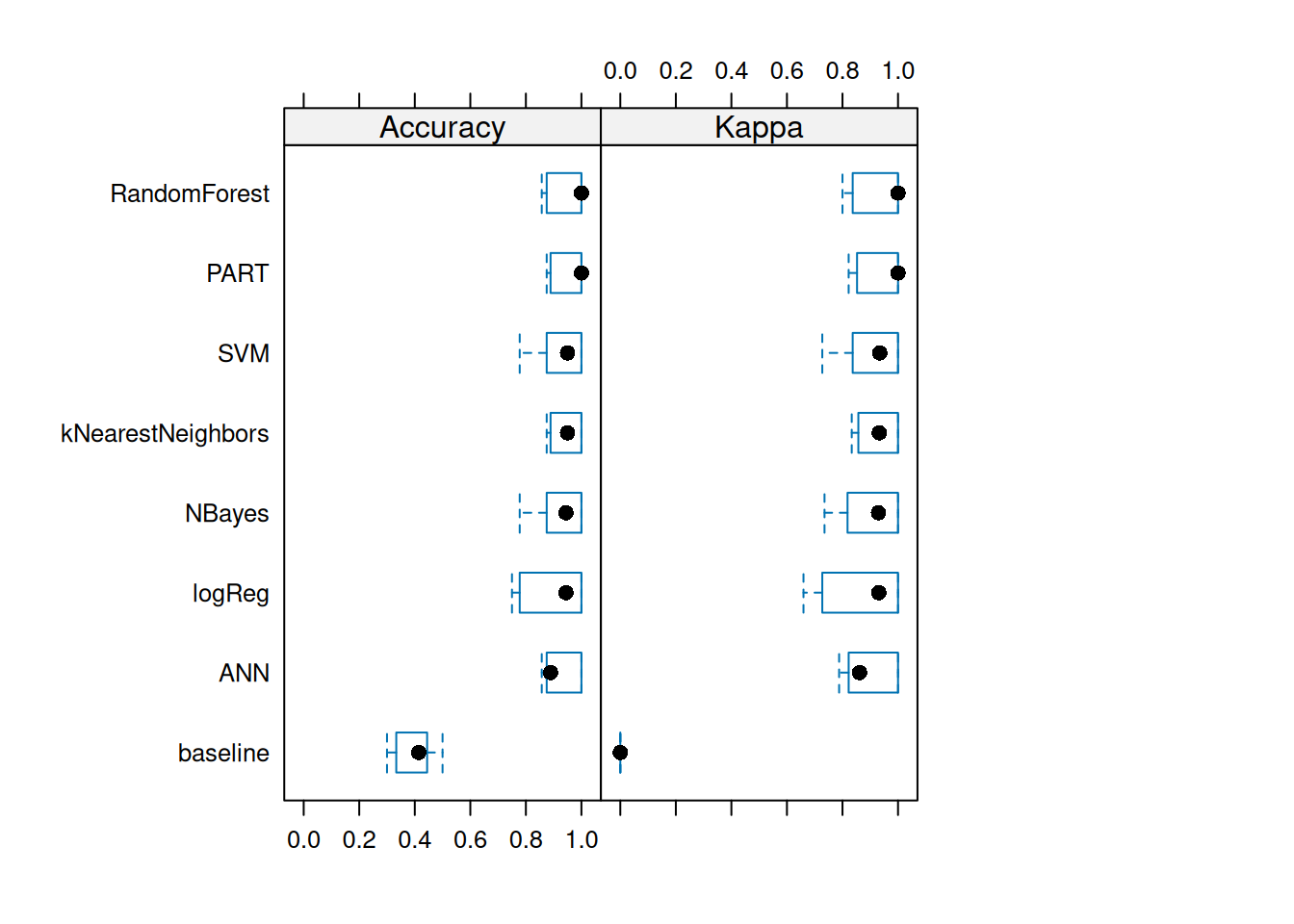
Compare paired resampling results for each metric. The output shows estimated differences and adjusted p-values. Because resampling folds are not independent, use these comparisons as descriptive evidence rather than definitive tests of which model is best. Bonferroni correction is applied for multiple comparisons.
difs <- diff(resamps)
summary(difs)
##
## Call:
## summary.diff.resamples(object = difs)
##
## p-value adjustment: bonferroni
## Upper diagonal: estimates of the difference
## Lower diagonal: p-value for H0: difference = 0
##
## Accuracy
##                   baseline PART     kNearestNeighbors
## baseline                   -0.54734 -0.53595
## PART              4.61e-08           0.01139
## kNearestNeighbors 1.30e-06 1
## NBayes            5.59e-06 1        1
## logReg            2.57e-05 1        1
## ANN               2.88e-06 1        1
## SVM               1.98e-06 1        1
## RandomForest      4.20e-07 1        1
##                   NBayes   logReg   ANN      SVM
## baseline          -0.52056 -0.49873 -0.51738 -0.52484
## PART               0.02679  0.04861  0.02996  0.02250
## kNearestNeighbors  0.01540  0.03722  0.01857  0.01111
## NBayes                      0.02183  0.00317 -0.00429
## logReg            1                 -0.01865 -0.02611
## ANN               1        1                 -0.00746
## SVM               1        1        1
## RandomForest      1        1        1        1
##                   RandomForest
## baseline          -0.54301
## PART               0.00433
## kNearestNeighbors -0.00706
## NBayes            -0.02246
## logReg            -0.04428
## ANN               -0.02563
## SVM               -0.01817
## RandomForest
##
## Kappa
##                   baseline PART     kNearestNeighbors
## baseline                   -0.93815 -0.92557
## PART              1.09e-09           0.01258
## kNearestNeighbors 1.07e-09 1
## NBayes            1.51e-08 1        1
## logReg            3.24e-07 1        1
## ANN               4.89e-09 1        1
## SVM               1.13e-08 1        1
## RandomForest      2.86e-09 1        1
##                   NBayes   logReg   ANN      SVM
## baseline          -0.90570 -0.87768 -0.89737 -0.91054
## PART               0.03245  0.06047  0.04078  0.02761
## kNearestNeighbors  0.01987  0.04789  0.02820  0.01503
## NBayes                      0.02802  0.00833 -0.00485
## logReg            1                 -0.01969 -0.03287
## ANN               1        1                 -0.01317
## SVM               1        1        1
## RandomForest      1        1        1        1
##                   RandomForest
## baseline          -0.93305
## PART               0.00510
## kNearestNeighbors -0.00748
## NBayes            -0.02735
## logReg            -0.05538
## ANN               -0.03568
## SVM               -0.02251
## RandomForest
The models have similar resampling performance except for the baseline. We select the random forest for illustration and evaluate it once on the held-out test set. The test set remains the final performance assessment.
pr <- predict(randomForestFit, Zoo_test)
pr
##  [1] mammal        fish          mollusc.et.al fish
##  [5] mammal        insect        mammal        mammal
##  [9] mammal        mammal        bird          mammal
## [13] mammal        bird          reptile       bird
## [17] mollusc.et.al bird
## 7 Levels: mammal bird reptile fish amphibian ... mollusc.et.al
Calculate the confusion matrix for the held-out test data.
confusionMatrix(pr, reference = Zoo_test$type)
## Confusion Matrix and Statistics
##
##                Reference
## Prediction      mammal bird reptile fish amphibian insect
##   mammal             8    0       0    0         0      0
##   bird               0    4       0    0         0      0
##   reptile            0    0       1    0         0      0
##   fish               0    0       0    2         0      0
##   amphibian          0    0       0    0         0      0
##   insect             0    0       0    0         0      1
##   mollusc.et.al      0    0       0    0         0      0
##                Reference
## Prediction      mollusc.et.al
##   mammal                    0
##   bird                      0
##   reptile                   0
##   fish                      0
##   amphibian                 0
##   insect                    0
##   mollusc.et.al             2
##
## Overall Statistics
##
##                Accuracy : 1
##                  95% CI : (0.815, 1)
##     No Information Rate : 0.444
##     P-Value [Acc > NIR] : 4.58e-07
##
##                   Kappa : 1
##
##  Mcnemar's Test P-Value : NA
##
## Statistics by Class:
##
##                      Class: mammal Class: bird
## Sensitivity                  1.000       1.000
## Specificity                  1.000       1.000
## Pos Pred Value               1.000       1.000
## Neg Pred Value               1.000       1.000
## Prevalence                   0.444       0.222
## Detection Rate               0.444       0.222
## Detection Prevalence         0.444       0.222
## Balanced Accuracy            1.000       1.000
##                      Class: reptile Class: fish
## Sensitivity                  1.0000       1.000
## Specificity                  1.0000       1.000
## Pos Pred Value               1.0000       1.000
## Neg Pred Value               1.0000       1.000
## Prevalence                   0.0556       0.111
## Detection Rate               0.0556       0.111
## Detection Prevalence         0.0556       0.111
## Balanced Accuracy            1.0000       1.000
##                      Class: amphibian Class: insect
## Sensitivity                        NA        1.0000
## Specificity                         1        1.0000
## Pos Pred Value                     NA        1.0000
## Neg Pred Value                     NA        1.0000
## Prevalence                          0        0.0556
## Detection Rate                      0        0.0556
## Detection Prevalence                0        0.0556
## Balanced Accuracy                  NA        1.0000
##                      Class: mollusc.et.al
## Sensitivity                         1.000
## Specificity                         1.000
## Pos Pred Value                      1.000
## Neg Pred Value                      1.000
## Prevalence                          0.111
## Detection Rate                      0.111
## Detection Prevalence                0.111
## Balanced Accuracy                   1.000
4.13 Class Imbalance
Class imbalance occurs when one class has substantially more observations than another. It can reduce performance on the minority class, especially when identifying that class is important (for example, detecting a rare disease). In a binary problem, the class of interest is often called the positive class. The examples below compare resampling, threshold adjustment, and cost-sensitive fitting.
For the examples, we will use the Zoo dataset.
library(rpart)
library(rpart.plot)
data(Zoo, package = "mlbench")
Check the class distribution before fitting a classifier.
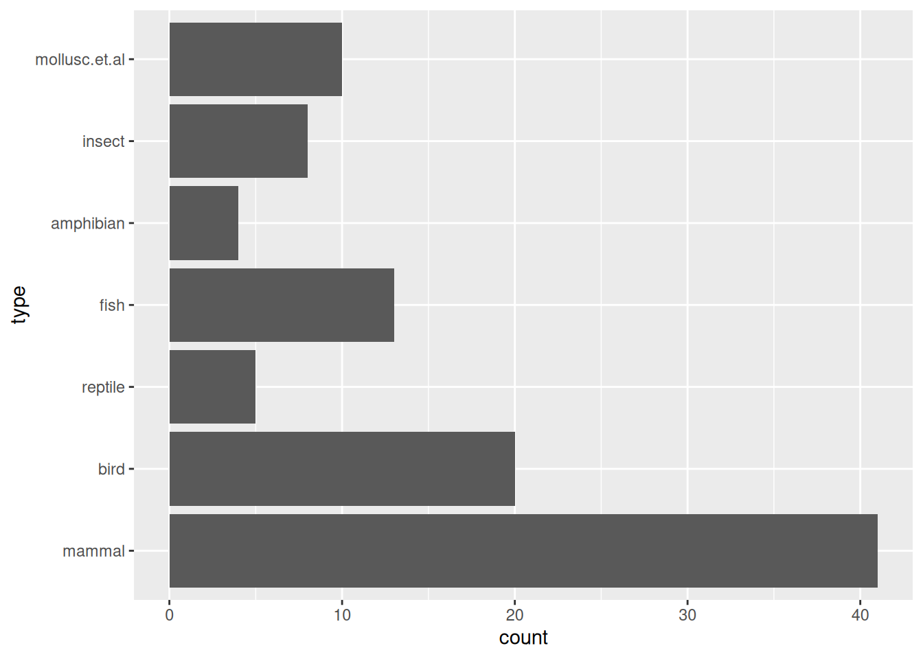
The Zoo data contain many mammals and few amphibians and reptiles. A classifier that favors the majority class may therefore have poor recall for the rarer classes, as the simple decision tree below illustrates.
tree_default <- Zoo |>
  rpart(type ~ ., data = _)
tree_default
## n= 101
##
## node), split, n, loss, yval, (yprob)
##       * denotes terminal node
##
##  1) root 101 60 mammal (0.41 0.2 0.05 0.13 0.04 0.079 0.099)
##    2) milk>=0.5 41  0 mammal (1 0 0 0 0 0 0) *
##    3) milk< 0.5 60 40 bird (0 0.33 0.083 0.22 0.067 0.13 0.17)
##      6) feathers>=0.5 20  0 bird (0 1 0 0 0 0 0) *
##      7) feathers< 0.5 40 27 fish (0 0 0.12 0.33 0.1 0.2 0.25)
##       14) fins>=0.5 13  0 fish (0 0 0 1 0 0 0) *
##       15) fins< 0.5 27 17 mollusc.et.al (0 0 0.19 0 0.15 0.3 0.37)
##         30) backbone>=0.5 9  4 reptile (0 0 0.56 0 0.44 0 0) *
##         31) backbone< 0.5 18  8 mollusc.et.al (0 0 0 0 0 0.44 0.56) *
library(rpart.plot)
rpart.plot(tree_default, extra = 2)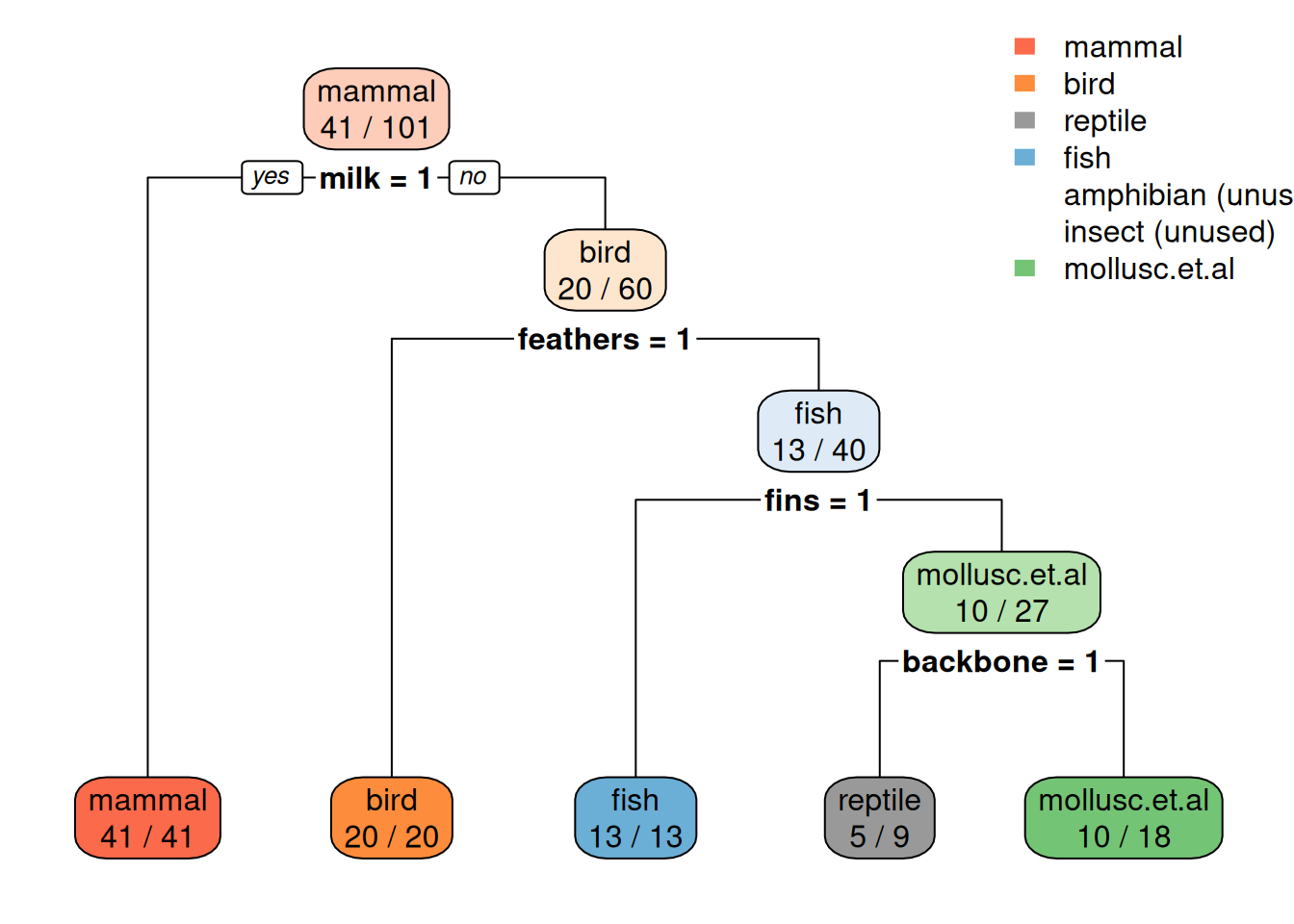
The resulting tree has no leaf nodes for these rare animal types, so it cannot predict them.
Predicting whether an animal is a reptile is a highly imbalanced binary classification problem. We set up this problem by changing the class variable to make it into a binary reptile/non-reptile classification problem.
Zoo_reptile <- Zoo |>
  mutate(type = factor(Zoo$type == "reptile",
                       levels = c(FALSE, TRUE),
                       labels = c("nonreptile", "reptile")))
Keep the class variable as a factor (categorical); otherwise rpart fits a
regression tree instead of a classification tree.
The class distribution shows that this classification problem is now highly imbalanced, with 5 reptiles and 96 non-reptiles.
summary(Zoo_reptile)
##     hair          feathers          eggs
##  Mode :logical   Mode :logical   Mode :logical
##  FALSE:58        FALSE:81        FALSE:42
##  TRUE :43        TRUE :20        TRUE :59
##
##
##
##     milk          airborne        aquatic
##  Mode :logical   Mode :logical   Mode :logical
##  FALSE:60        FALSE:77        FALSE:65
##  TRUE :41        TRUE :24        TRUE :36
##
##
##
##   predator        toothed         backbone
##  Mode :logical   Mode :logical   Mode :logical
##  FALSE:45        FALSE:40        FALSE:18
##  TRUE :56        TRUE :61        TRUE :83
##
##
##
##   breathes        venomous          fins
##  Mode :logical   Mode :logical   Mode :logical
##  FALSE:21        FALSE:93        FALSE:84
##  TRUE :80        TRUE :8         TRUE :17
##
##
##
##       legs         tail          domestic
##  Min.   :0.00   Mode :logical   Mode :logical
##  1st Qu.:2.00   FALSE:26        FALSE:88
##  Median :4.00   TRUE :75        TRUE :13
##  Mean   :2.84
##  3rd Qu.:4.00
##  Max.   :8.00
##   catsize                type
##  Mode :logical   nonreptile:96
##  FALSE:57        reptile   : 5
##  TRUE :44
##
##
## 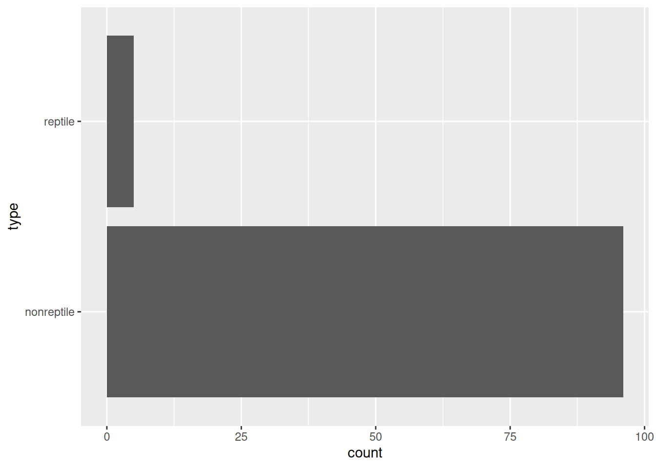
The graph shows that a non-reptile is about 20 times as common as a reptile in this dataset. We will compare several ways to address this imbalance.
We split the data into training and test sets so we can evaluate each approach on observations not used for fitting. A 50/50 split increases the chance that the small test set includes reptiles. Estimates remain highly uncertain because there are only five reptiles in total.
set.seed(1234)

inTrain <- createDataPartition(y = Zoo_reptile$type, p = .5)[[1]]
training_reptile <- Zoo_reptile |> slice(inTrain)
testing_reptile <- Zoo_reptile |> slice(-inTrain)
4.13.1 Option 1: Use the Original Class Distribution
fit <- training_reptile |>
  train(type ~ .,
        data = _,
        method = "rpart",
        trControl = trainControl(method = "cv"))
## Warning in nominalTrainWorkflow(x = x, y = y, wts =
## weights, info = trainInfo, : There were missing values in
## resampled performance measures.
Warnings: “There were missing values in resampled performance measures.” means that some test folds used in hyper parameter tuning did not contain examples of both classes. This is very likely with strong class imbalance and small datasets.
fit
## CART
##
## 51 samples
## 16 predictors
##  2 classes: 'nonreptile', 'reptile'
##
## No pre-processing
## Resampling: Cross-Validated (10 fold)
## Summary of sample sizes: 46, 47, 46, 46, 45, 46, ...
## Resampling results:
##
##   Accuracy  Kappa
##   0.9467    0
##
## Tuning parameter 'cp' was held constant at a value of 0
rpart.plot(fit$finalModel, extra = 2)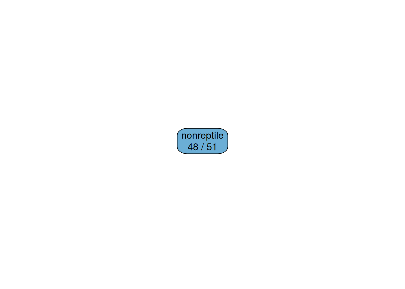
The tree predicts everything as non-reptile. Have a look at the error on the test set.
confusionMatrix(data = predict(fit, testing_reptile),
                ref = testing_reptile$type, positive = "reptile")
## Confusion Matrix and Statistics
##
##             Reference
## Prediction   nonreptile reptile
##   nonreptile         48       2
##   reptile             0       0
##
##                Accuracy : 0.96
##                  95% CI : (0.863, 0.995)
##     No Information Rate : 0.96
##     P-Value [Acc > NIR] : 0.677
##
##                   Kappa : 0
##
##  Mcnemar's Test P-Value : 0.480
##
##             Sensitivity : 0.00
##             Specificity : 1.00
##          Pos Pred Value :  NaN
##          Neg Pred Value : 0.96
##              Prevalence : 0.04
##          Detection Rate : 0.00
##    Detection Prevalence : 0.00
##       Balanced Accuracy : 0.50
##
##        'Positive' Class : reptile
##
Accuracy equals the no-information rate and kappa is zero. Sensitivity is also zero: the model identifies no reptiles. When missing a positive case is more costly than misclassifying a negative, accuracy alone is not an adequate metric. Sensitivity, specificity, and the costs of each type of error should also be considered.
Note: The positive class value (the one that you want to detect) is
set manually to reptile using positive = "reptile". Otherwise
sensitivity/specificity will not be correctly calculated.
4.13.2 Option 2: Upsample Within Resampling
A common approach is to upsample the minority class by drawing observations
with replacement. Upsampling must happen within each resampling iteration;
otherwise, duplicate observations can appear in both the fold used for fitting
and the fold used for validation. caret supports this through the sampling
argument to trainControl() (see the caret subsampling
guide).
set.seed(1000) # for repeatability

fit <- training_reptile |>
  train(type ~ .,
        data = _,
        method = "rpart",
        trControl = trainControl(method = "cv", sampling = "up"),
        control = rpart.control(minsplit = 5))
## Warning in nominalTrainWorkflow(x = x, y = y, wts =
## weights, info = trainInfo, : There were missing values in
## resampled performance measures.
fit
## CART
##
## 51 samples
## 16 predictors
##  2 classes: 'nonreptile', 'reptile'
##
## No pre-processing
## Resampling: Cross-Validated (10 fold)
## Summary of sample sizes: 46, 46, 46, 45, 46, 46, ...
## Addtional sampling using up-sampling
##
## Resampling results:
##
##   Accuracy  Kappa
##   0.8667    0
##
## Tuning parameter 'cp' was held constant at a value of 0
rpart.plot(fit$finalModel, extra = 2)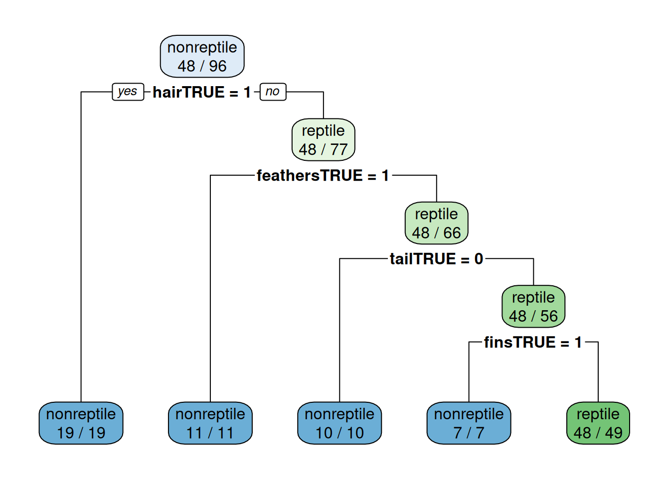
Upsampling is applied only to each analysis fold; validation folds and the held-out test set keep the observed class distribution. Evaluate the fitted model on that untouched test set:
confusionMatrix(data = predict(fit, testing_reptile),
                ref = testing_reptile$type, positive = "reptile")
## Confusion Matrix and Statistics
##
##             Reference
## Prediction   nonreptile reptile
##   nonreptile         47       0
##   reptile             1       2
##
##                Accuracy : 0.98
##                  95% CI : (0.894, 0.999)
##     No Information Rate : 0.96
##     P-Value [Acc > NIR] : 0.4
##
##                   Kappa : 0.79
##
##  Mcnemar's Test P-Value : 1.0
##
##             Sensitivity : 1.000
##             Specificity : 0.979
##          Pos Pred Value : 0.667
##          Neg Pred Value : 1.000
##              Prevalence : 0.040
##          Detection Rate : 0.040
##    Detection Prevalence : 0.060
##       Balanced Accuracy : 0.990
##
##        'Positive' Class : reptile
##
Compare accuracy, sensitivity, and specificity with the unresampled model. Because the test set contains very few reptiles, each metric can change substantially if even one observation is classified differently.
Upsampling changes the class balance seen during fitting, but it does not directly specify the relative costs of false positives and false negatives. Choose a decision threshold or use a cost-sensitive method when you need to express that tradeoff; see Options 3 and 4.
4.13.3 Option 3: Build A Larger Tree and use Predicted Probabilities
We increase tree complexity and require fewer observations to split a node.
Here we tune using the area under the ROC curve (ROC AUC). twoClassSummary
requires class probabilities, which we also need for the threshold example
below. The tree is still fit using its standard splitting criterion; ROC AUC
is the metric used to select the tuning parameter.
fit <- training_reptile |>
  train(type ~ .,
        data = _,
        method = "rpart",
        tuneLength = 10,
        trControl = trainControl(
                        method = "cv",
                        classProbs = TRUE,  ## for predict with type="prob"
                        summaryFunction=twoClassSummary),  ## for ROC
        metric = "ROC",
        control = rpart.control(minsplit = 3))
## Warning in nominalTrainWorkflow(x = x, y = y, wts =
## weights, info = trainInfo, : There were missing values in
## resampled performance measures.
fit
## CART
##
## 51 samples
## 16 predictors
##  2 classes: 'nonreptile', 'reptile'
##
## No pre-processing
## Resampling: Cross-Validated (10 fold)
## Summary of sample sizes: 45, 46, 46, 46, 46, 46, ...
## Resampling results:
##
##   ROC     Sens  Spec
##   0.3667  0.94  0
##
## Tuning parameter 'cp' was held constant at a value of 0
rpart.plot(fit$finalModel, extra = 2)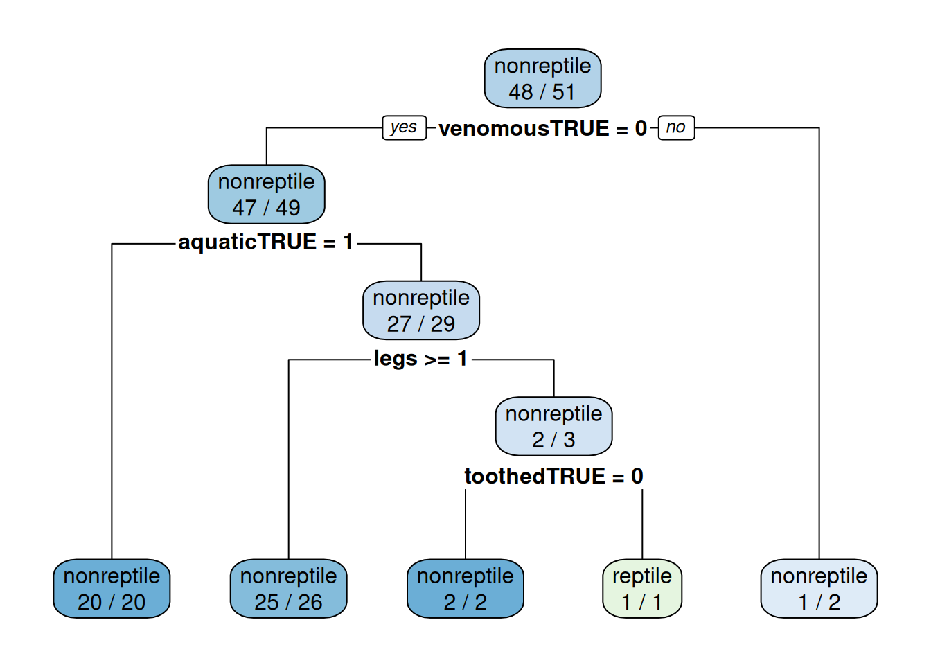
confusionMatrix(data = predict(fit, testing_reptile),
                ref = testing_reptile$type, positive = "reptile")
## Confusion Matrix and Statistics
##
##             Reference
## Prediction   nonreptile reptile
##   nonreptile         48       2
##   reptile             0       0
##
##                Accuracy : 0.96
##                  95% CI : (0.863, 0.995)
##     No Information Rate : 0.96
##     P-Value [Acc > NIR] : 0.677
##
##                   Kappa : 0
##
##  Mcnemar's Test P-Value : 0.480
##
##             Sensitivity : 0.00
##             Specificity : 1.00
##          Pos Pred Value :  NaN
##          Neg Pred Value : 0.96
##              Prevalence : 0.04
##          Detection Rate : 0.00
##    Detection Prevalence : 0.00
##       Balanced Accuracy : 0.50
##
##        'Positive' Class : reptile
##
Note: Accuracy is close to the no-information rate on this small dataset.
4.13.3.1 Create A Biased Classifier
We can lower the classification threshold to identify more reptiles at the cost of misclassifying more non-reptiles. For a binary classifier, the default threshold is often 0.5. Lowering it predicts more positives, typically increasing sensitivity at the cost of specificity. The 0.01 threshold below is illustrative; a real threshold should be selected using validation data and application-specific costs.
prob <- predict(fit, testing_reptile, type = "prob")
tail(prob)
##      nonreptile reptile
## tuna     1.0000 0.00000
## vole     0.9615 0.03846
## wasp     0.5000 0.50000
## wolf     0.9615 0.03846
## worm     1.0000 0.00000
## wren     0.9615 0.03846
pred <- ifelse(prob[,"reptile"] >= 0.01, "reptile", "nonreptile") |>
  as.factor()

confusionMatrix(data = pred,
                ref = testing_reptile$type, positive = "reptile")
## Confusion Matrix and Statistics
##
##             Reference
## Prediction   nonreptile reptile
##   nonreptile         13       0
##   reptile            35       2
##
##                Accuracy : 0.3
##                  95% CI : (0.179, 0.446)
##     No Information Rate : 0.96
##     P-Value [Acc > NIR] : 1
##
##                   Kappa : 0.029
##
##  Mcnemar's Test P-Value : 9.08e-09
##
##             Sensitivity : 1.0000
##             Specificity : 0.2708
##          Pos Pred Value : 0.0541
##          Neg Pred Value : 1.0000
##              Prevalence : 0.0400
##          Detection Rate : 0.0400
##    Detection Prevalence : 0.7400
##       Balanced Accuracy : 0.6354
##
##        'Positive' Class : reptile
##
This lower threshold trades accuracy and specificity for sensitivity on this split. Accuracy treats all errors equally and does not capture the cost of missing a reptile.
4.13.3.2 Plot the ROC Curve
Since we have a binary classification problem and a classifier that predicts a probability for an observation to be a reptile, we can also use a receiver operating characteristic (ROC) curve. The ROC curve shows sensitivity against the false-positive rate over different probability thresholds. Its area (ROC AUC) summarizes ranking performance: 0.5 corresponds to chance ranking and 1 to perfect ranking. It does not select an operating threshold or account for application-specific error costs.
library("pROC")
## Type 'citation("pROC")' for a citation.
##
## Attaching package: 'pROC'
## The following objects are masked from 'package:stats':
##
##     cov, smooth, var
r <- roc(testing_reptile$type == "reptile", prob[,"reptile"])
## Setting levels: control = FALSE, case = TRUE
## Setting direction: controls < cases
r
##
## Call:
## roc.default(response = testing_reptile$type == "reptile", predictor = prob[,     "reptile"])
##
## Data: prob[, "reptile"] in 48 controls (testing_reptile$type == "reptile" FALSE) < 2 cases (testing_reptile$type == "reptile" TRUE).
## Area under the curve: 0.766
ggroc(r) + geom_abline(intercept = 1, slope = 1, color = "darkgrey")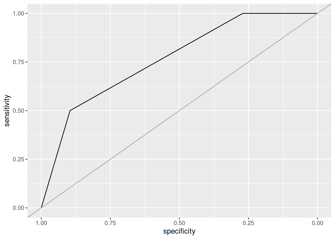
This ROC curve is calculated on the test set for illustration. Do not choose a threshold from this curve and then report performance on the same test set; use validation data to choose the threshold and reserve the test set for the final evaluation.
4.13.4 Option 4: Use a Cost-Sensitive Classifier
The CART implementation in rpart accepts a loss matrix through the loss
parameter. Rows represent actual classes and columns represent predicted
classes. The diagonal entries (correct predictions) have zero cost. We assign
a false negative a cost of 100 and a false positive a cost of 1:
                 predicted
actual       nonreptile reptile
nonreptile       0         1
reptile         100        0
cost <- matrix(c(
  0,   1,
  100, 0
), byrow = TRUE, nrow = 2)
cost
##      [,1] [,2]
## [1,]    0    1
## [2,]  100    0
fit <- training_reptile |>
  train(type ~ .,
        data = _,
        method = "rpart",
        parms = list(loss = cost),
        trControl = trainControl(method = "cv"))
## Warning in nominalTrainWorkflow(x = x, y = y, wts =
## weights, info = trainInfo, : There were missing values in
## resampled performance measures.
The warning “There were missing values in resampled performance measures” means that some validation folds did not contain both classes. With only a few reptiles, this can make cross-validation metrics unstable or undefined.
fit
## CART
##
## 51 samples
## 16 predictors
##  2 classes: 'nonreptile', 'reptile'
##
## No pre-processing
## Resampling: Cross-Validated (10 fold)
## Summary of sample sizes: 46, 46, 47, 45, 46, 45, ...
## Resampling results:
##
##   Accuracy  Kappa
##   0.545     -0.002273
##
## Tuning parameter 'cp' was held constant at a value of 0
rpart.plot(fit$finalModel, extra = 2)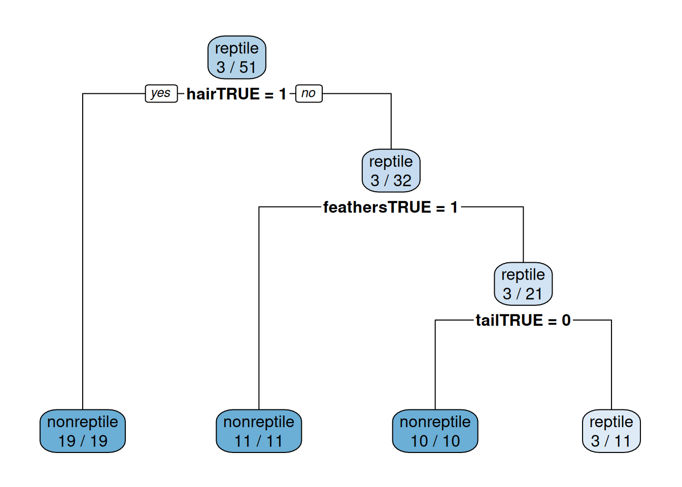
confusionMatrix(data = predict(fit, testing_reptile),
                ref = testing_reptile$type, positive = "reptile")
## Confusion Matrix and Statistics
##
##             Reference
## Prediction   nonreptile reptile
##   nonreptile         39       0
##   reptile             9       2
##
##                Accuracy : 0.82
##                  95% CI : (0.686, 0.914)
##     No Information Rate : 0.96
##     P-Value [Acc > NIR] : 0.99998
##
##                   Kappa : 0.257
##
##  Mcnemar's Test P-Value : 0.00766
##
##             Sensitivity : 1.000
##             Specificity : 0.812
##          Pos Pred Value : 0.182
##          Neg Pred Value : 1.000
##              Prevalence : 0.040
##          Detection Rate : 0.040
##    Detection Prevalence : 0.220
##       Balanced Accuracy : 0.906
##
##        'Positive' Class : reptile
##
In this split, the high false-negative cost results in a classifier that identifies all reptiles. This result is specific to this small split; it does not guarantee perfect sensitivity on new data.
Cost-sensitive fitting is useful when error costs are known and the chosen algorithm supports them. Other approaches include adjusting a decision threshold or using weighted loss functions; availability depends on the model and software implementation.
4.14 Comparing Decision Boundaries of Popular Classification Techniques*
Classifiers create decision boundaries to discriminate between classes. Different classifiers are able to create different shapes of decision boundaries (e.g., some are strictly linear) and thus some classifiers may perform better for certain datasets. In this section, we visualize the decision boundaries found by several popular classification methods.
The following function defines a plot that adds the decision boundary (black lines) and the difference between the classification probability of the two best classes (color intensity; indifference is 0 shown as white) by evaluating the classifier at evenly spaced grid points. Note that low resolution will make evaluation faster but it also will make the decision boundary look like it has small steps even if it is a straight line.
decisionplot <- function(model, data, class_var,
  predict_type = c("class", "prob"), resolution = 3 * 72) {
  # resolution is set to 72 dpi for 3 inches wide images.

  y <- data |> pull(class_var)
  x <- data |> dplyr::select(-all_of(class_var))

  # resubstitution accuracy
  prediction <- predict(model, x, type = predict_type[1])

  # LDA returns a list
  if(is.list(prediction)) prediction <- prediction$class

  prediction <- factor(prediction, levels = levels(y))
  cm <- confusionMatrix(data = prediction,
                        reference = y)
  acc <- cm$overall["Accuracy"]

  # evaluate model on a grid
  r <- sapply(x[, 1:2], range, na.rm = TRUE)
  xs <- seq(r[1,1], r[2,1], length.out = resolution)
  ys <- seq(r[1,2], r[2,2], length.out = resolution)
  g <- cbind(rep(xs, each = resolution), rep(ys,
                                             time = resolution))
  colnames(g) <- colnames(r)
  g <- as_tibble(g)

  # guess how to get class labels from predict
  # (unfortunately not very consistent between models)
  cl <- predict(model, g, type = predict_type[1])

  prob <- NULL
  if(is.list(cl)) { # LDA returns a list
    prob <- cl$posterior
    cl <- cl$class
  } else if (inherits(model, "svm"))
    prob <- attr(predict(model, g, probability = TRUE), "probabilities")
  else
    if(!is.na(predict_type[2]))
      try(prob <- predict(model, g, type = predict_type[2]))

  # We visualize the difference in probability/score between
  # the winning class and the second best class. We only use
  # probability if the classifier's predict function supports it.
  delta_prob <- 1
  if(!is.null(prob))

    try({
      if (any(rowSums(prob) != 1))
        prob <- cbind(prob, 1 - rowSums(prob))

      max_prob <- t(apply(prob, MARGIN = 1, sort, decreasing = TRUE))
      delta_prob <- max_prob[,1] - max_prob[,2]
    }, silent = TRUE)

  cl <- factor(cl, levels = levels(y))

  g <- g |> add_column(prediction = cl,
                       delta_prob = delta_prob)

  ggplot(g, mapping = aes(
    x = .data[[colnames(g)[1]]],
    y = .data[[colnames(g)[2]]])) +
    geom_raster(mapping = aes(fill = prediction,
                              alpha = delta_prob)) +
    geom_contour(mapping = aes(z = as.numeric(prediction)),
      bins = length(levels(cl)),
      linewidth = .5,
      color = "black") +
    geom_point(data = data, mapping =  aes(
      x = .data[[colnames(data)[1]]],
      y = .data[[colnames(data)[2]]],
      shape = .data[[class_var]]),
      alpha = .7) +
    scale_alpha_continuous(range = c(0,1),
                           limits = c(0,1)) +
    labs(subtitle = paste("Training accuracy:", round(acc, 2)))
}
4.14.1 Iris Dataset
For easier visualization, we use two dimensions of the Iris dataset.
set.seed(1000)
data(iris)
iris <- as_tibble(iris)

x <- iris |> dplyr::select(Sepal.Length, Sepal.Width, Species)
# Note: package MASS overwrites the select function.

x
## # A tibble: 150 × 3
##    Sepal.Length Sepal.Width Species
##           <dbl>       <dbl> <fct>
##  1          5.1         3.5 setosa
##  2          4.9         3   setosa
##  3          4.7         3.2 setosa
##  4          4.6         3.1 setosa
##  5          5           3.6 setosa
##  6          5.4         3.9 setosa
##  7          4.6         3.4 setosa
##  8          5           3.4 setosa
##  9          4.4         2.9 setosa
## 10          4.9         3.1 setosa
## # ℹ 140 more rows
ggplot(x, aes(x = Sepal.Length,
              y = Sepal.Width,
              fill = Species)) +
  stat_density_2d(geom = "polygon",
                  aes(alpha = after_stat(level))) +
  geom_point()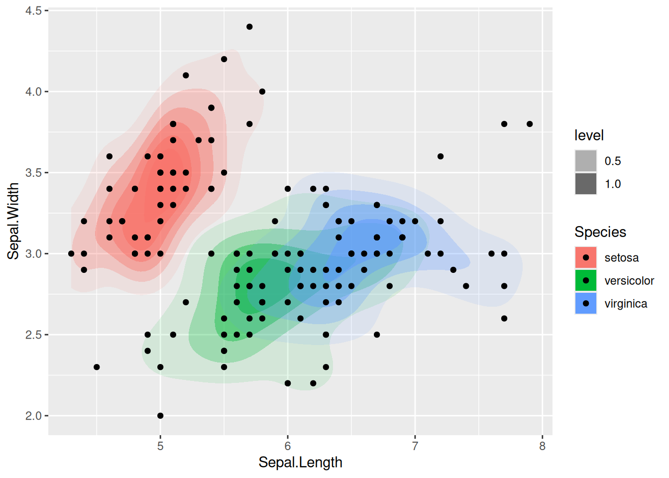
This is the original data.
Color is used to show the density.
Note that there is some overplotting with several points in the same position.
You could use geom_jitter() instead of geom_point().
4.14.1.1 Nearest Neighbor Classifier
We try several values for \(k\).
model <- x |> caret::knn3(Species ~ ., data = _, k = 1)
decisionplot(model, x, class_var = "Species") +
  labs(title = "kNN (1 neighbor)")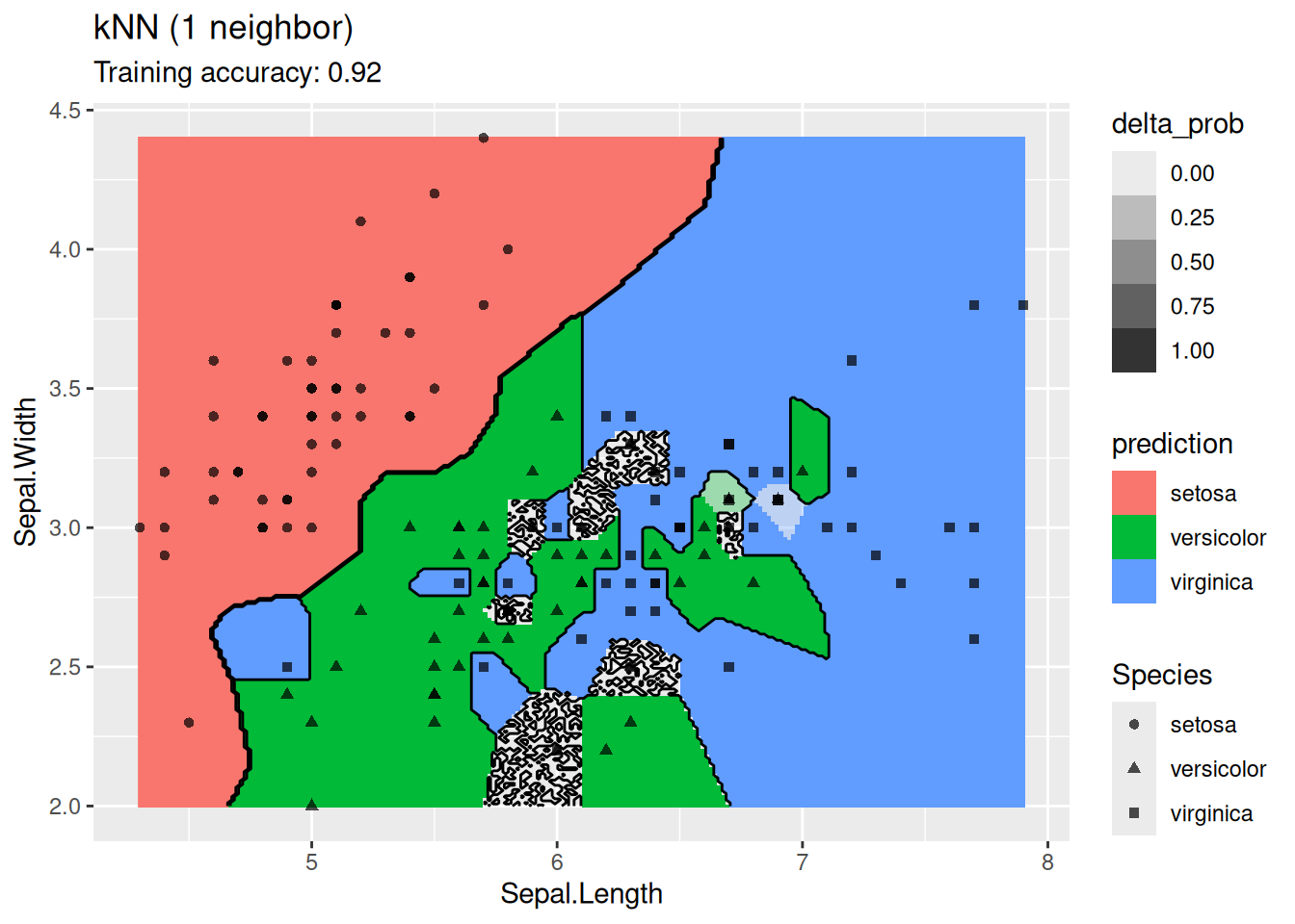
model <- x |> caret::knn3(Species ~ ., data = _, k = 3)
decisionplot(model, x, class_var = "Species") +
  labs(title = "kNN (3 neighbors)")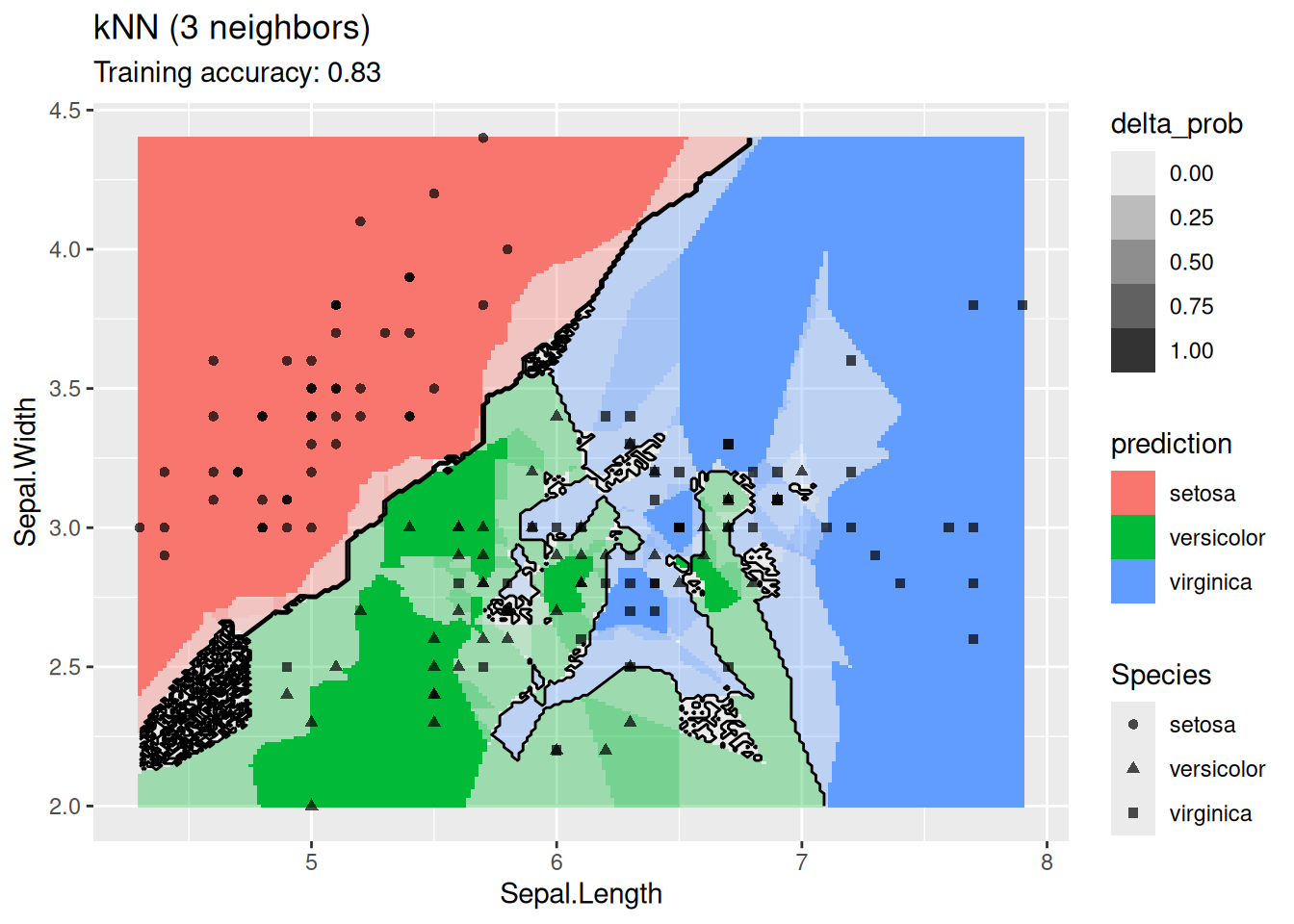
model <- x |> caret::knn3(Species ~ ., data = _, k = 9)
decisionplot(model, x, class_var = "Species") +
  labs(title = "kNN (9 neighbors)")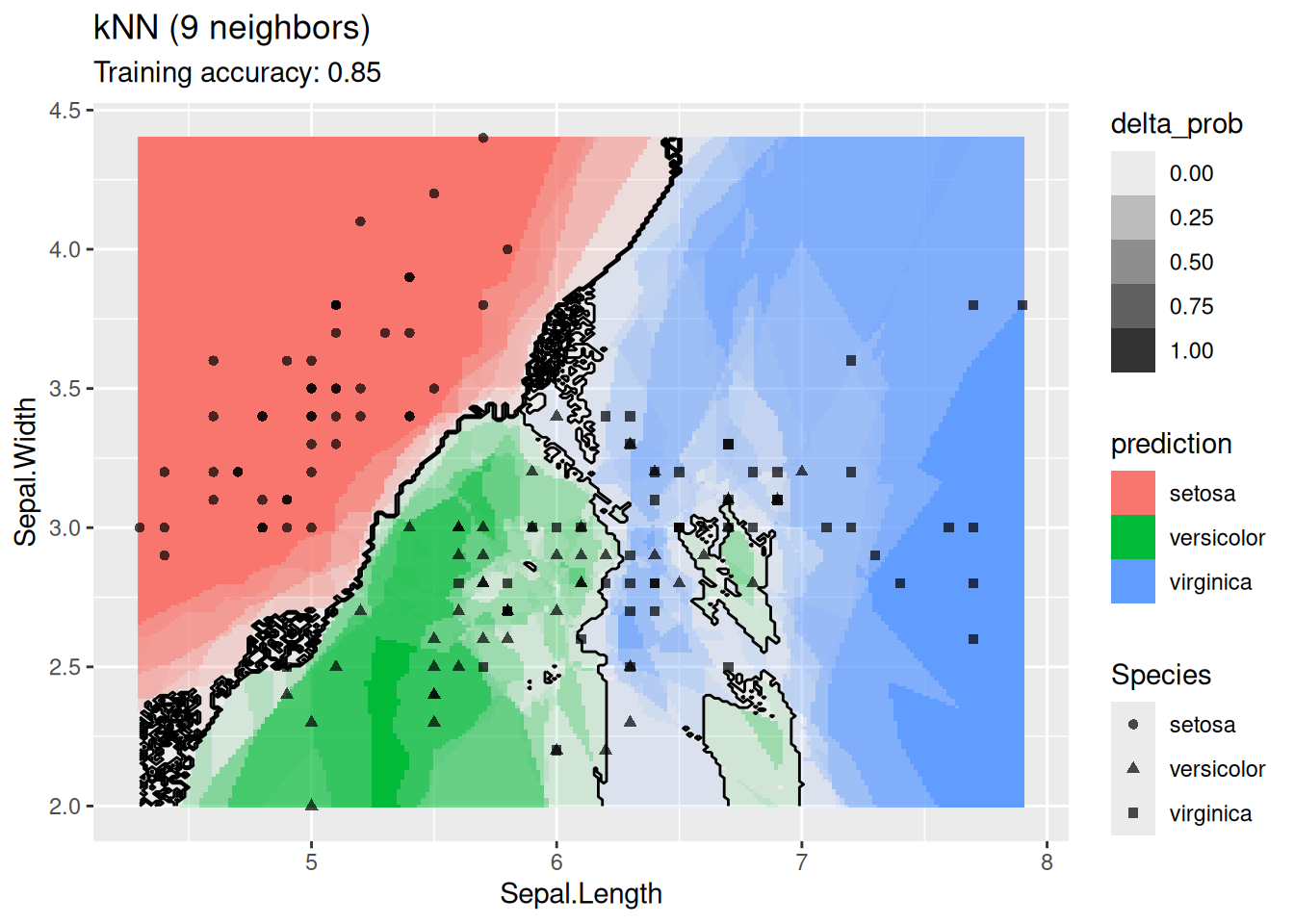
Increasing \(k\) smooths the decision boundary. At \(k=1\), we see white areas around points where flowers of two classes are in the same spot. Here, the algorithm randomly chooses a class during prediction resulting in the meandering decision boundary. The predictions in that area are not stable and every time we ask for a class, we may get a different class.
Note: The crazy lines in white areas are an artifact of the visualization. Here the classifier randomly selects a class.
4.14.1.2 Naive Bayes Classifier
Use a Gaussian naive Bayes classifier.
model <- x |> e1071::naiveBayes(Species ~ ., data = _)
decisionplot(model, x, class_var = "Species",
             predict_type = c("class", "raw")) +
  labs(title = "Naive Bayes")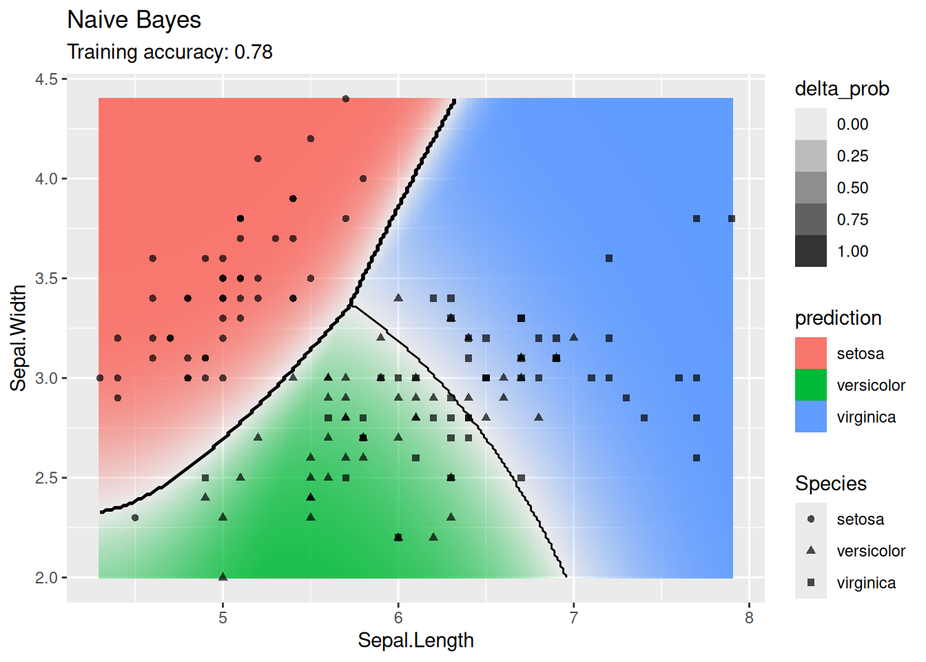
The GBN finds a good model with the advantage that no hyperparameters are needed.
4.14.1.3 Linear Discriminant Analysis
LDA finds linear decision boundaries.
model <- x |> MASS::lda(Species ~ ., data = _)
decisionplot(model, x, class_var = "Species") +
  labs(title = "LDA")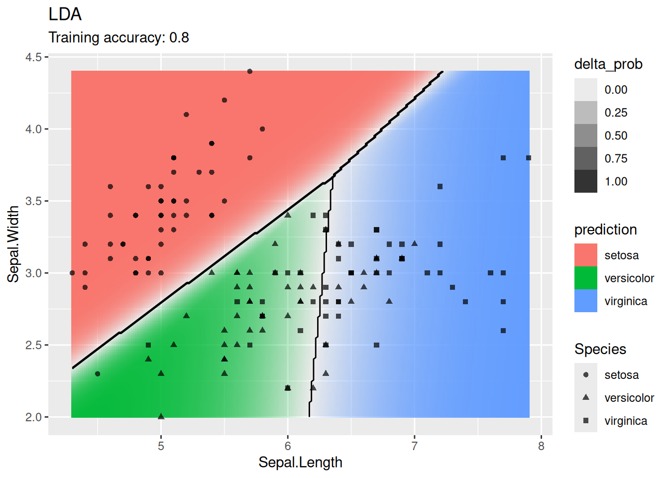
Linear decision boundaries work for this dataset so LDA works well.
4.14.1.4 Multinomial Logistic Regression
Multinomial logistic regression is an extension of logistic regression to problems with more than two classes.
model <- x |> nnet::multinom(Species ~., data = _)
## # weights:  12 (6 variable)
## initial  value 164.791843
## iter  10 value 62.715967
## iter  20 value 59.808291
## iter  30 value 55.445984
## iter  40 value 55.375704
## iter  50 value 55.346472
## iter  60 value 55.301707
## iter  70 value 55.253532
## iter  80 value 55.243230
## iter  90 value 55.230241
## iter 100 value 55.212479
## final  value 55.212479
## stopped after 100 iterations
decisionplot(model, x, class_var = "Species") +
  labs(titel = "Multinomial Logistic Regression")
## Ignoring unknown labels:
## • titel : "Multinomial Logistic Regression"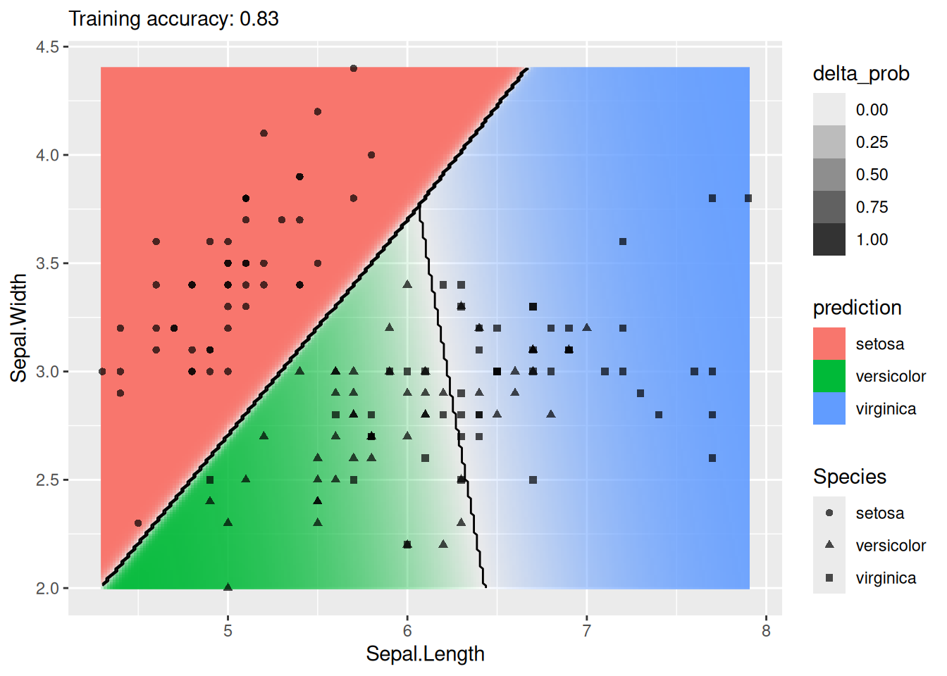
4.14.1.5 Decision Trees
Compare different types of decision trees.
model <- x |> rpart::rpart(Species ~ ., data = _)
decisionplot(model, x, class_var = "Species") +
  labs(title = "CART")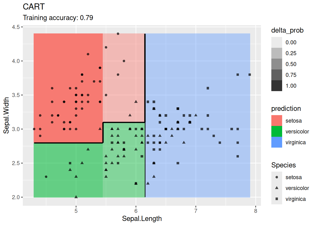
model <- x |> rpart::rpart(Species ~ ., data = _,
  control = rpart::rpart.control(cp = 0.001, minsplit = 1))
decisionplot(model, x, class_var = "Species") +
  labs(title = "CART (overfitting)")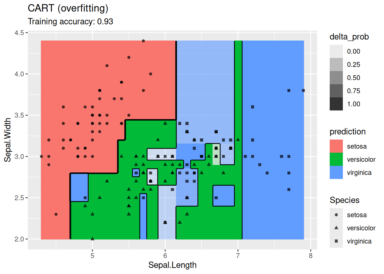
model <- x |> C50::C5.0(Species ~ ., data = _)
decisionplot(model, x, class_var = "Species") +
  labs(title = "C5.0")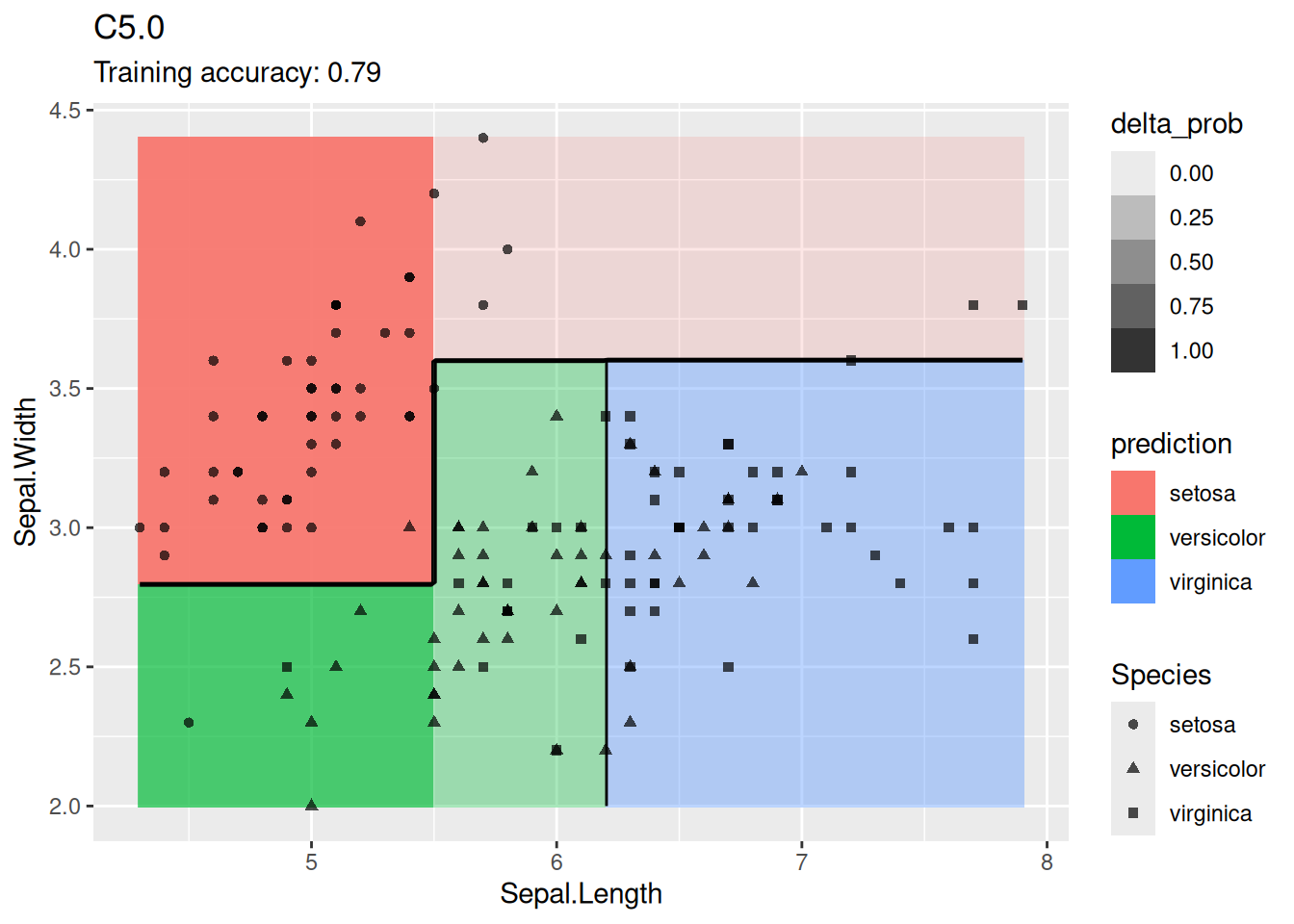
4.14.1.6 Ensemble: Random Forest
Use an ensemble method.
model <- x |> randomForest::randomForest(Species ~ ., data = _)
decisionplot(model, x, class_var = "Species") +
  labs(title = "Random Forest")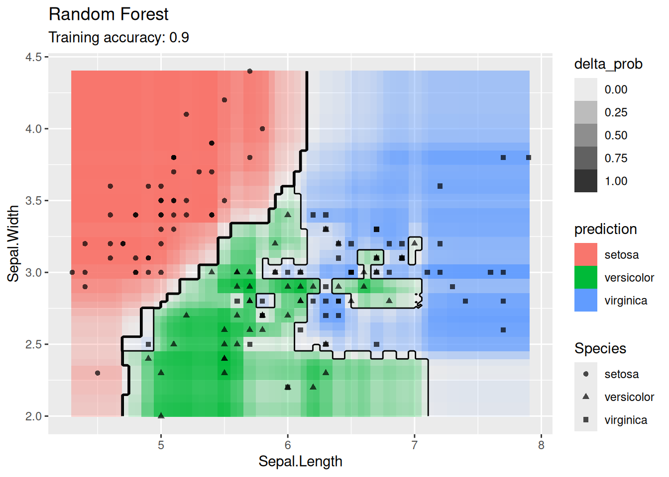
For the default settings for Random forest, the model seems to overfit the training data. More data would probably alleviate this issue.
4.14.1.7 Support Vector Machine
Compare SVMs with different kernel functions.
model <- x |> e1071::svm(Species ~ ., data = _,
                         kernel = "linear", probability = TRUE)
decisionplot(model, x, class_var = "Species") +
  labs(title = "SVM (linear kernel)")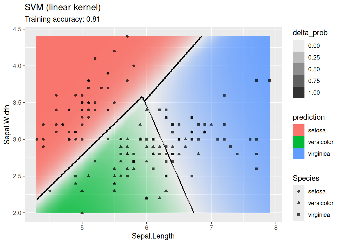
model <- x |> e1071::svm(Species ~ ., data = _,
                         kernel = "radial", probability = TRUE)
decisionplot(model, x, class_var = "Species") +
  labs(title = "SVM (radial kernel)")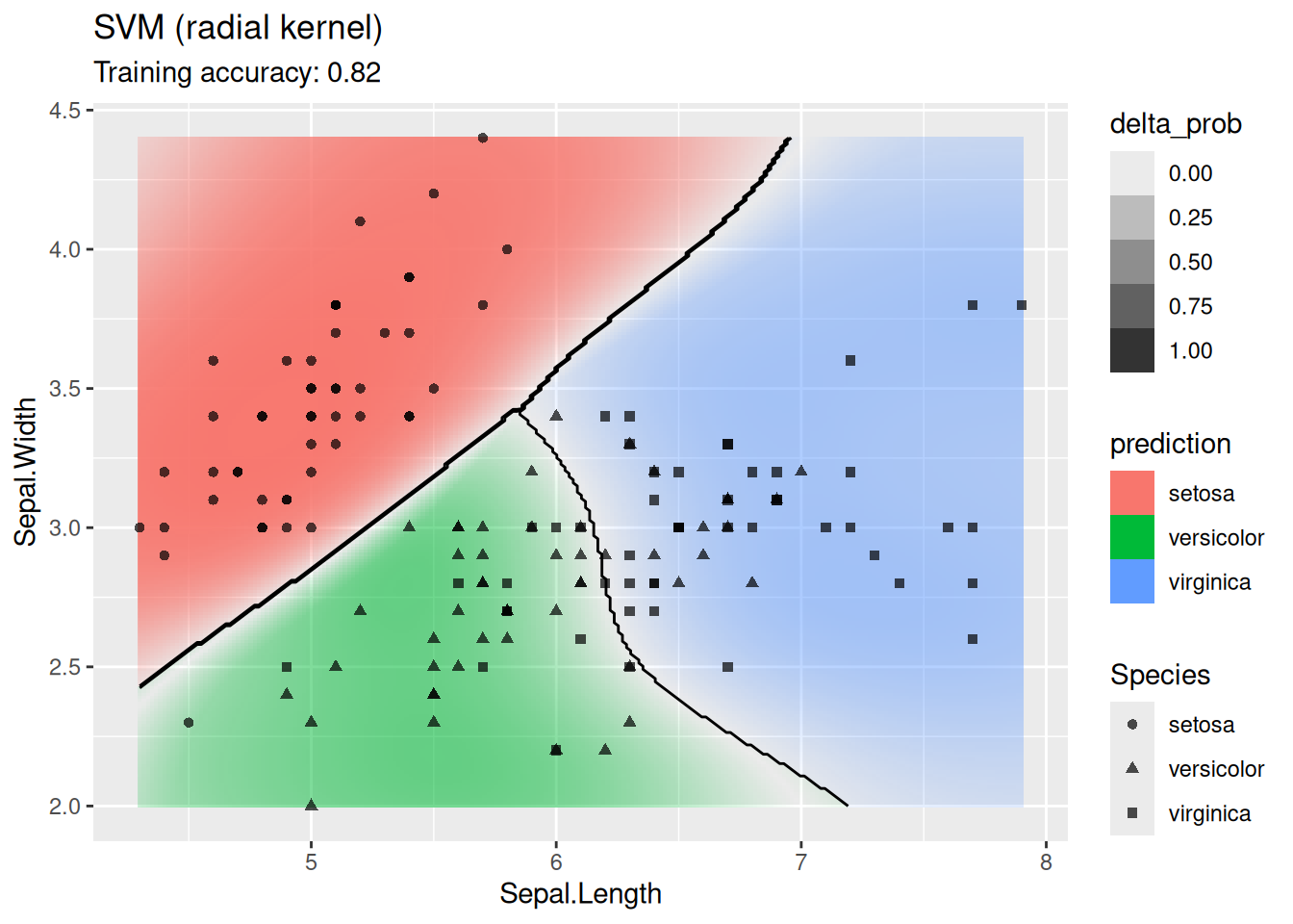
model <- x |> e1071::svm(Species ~ ., data = _,
                         kernel = "polynomial", probability = TRUE)
decisionplot(model, x, class_var = "Species") +
  labs(title = "SVM (polynomial kernel)")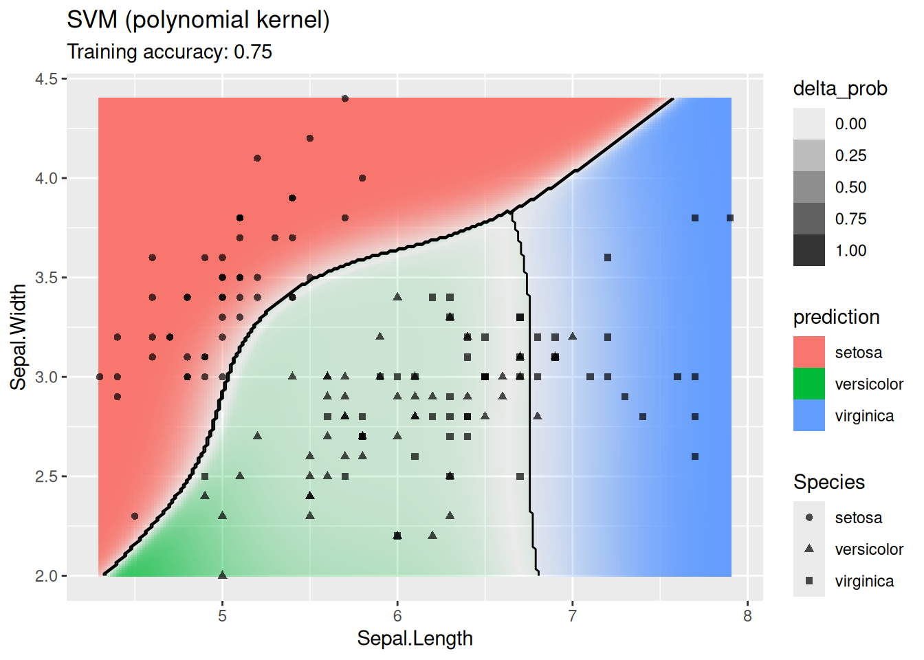
model <- x |> e1071::svm(Species ~ ., data = _,
                         kernel = "sigmoid", probability = TRUE)
decisionplot(model, x, class_var = "Species") +
  labs(title = "SVM (sigmoid kernel)")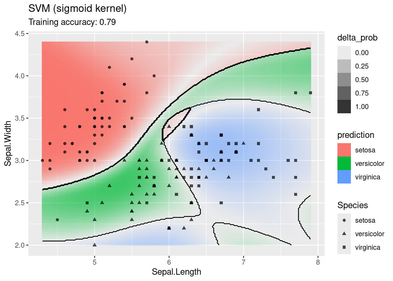
The linear SVM (without a kernel) produces straight lines and works well on the iris data. Most kernels do also well, only the sigmoid kernel seems to find a very strange decision boundary which indicates that the data does not have a linear decision boundary in the projected space.
4.14.1.8 Single Layer Feed-forward Neural Networks
Use a simple network with one hidden layer. We will try a different number of neurons for the hidden layer.
set.seed(1234)

model <- x |> nnet::nnet(Species ~ ., data = _,
                        size = 1, trace = FALSE)
decisionplot(model, x, class_var  = "Species",
             predict_type = c("class", "raw")) +
  labs(title = "ANN (1 neuron)")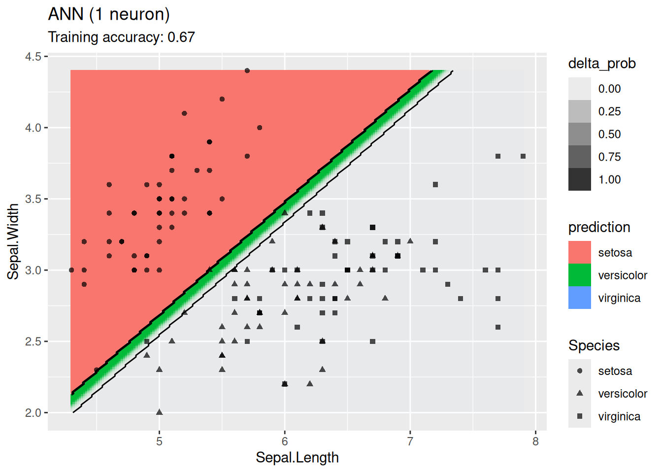
model <- x |> nnet::nnet(Species ~ ., data = _,
                        size = 2, trace = FALSE)
decisionplot(model, x, class_var  = "Species",
             predict_type = c("class", "raw")) +
  labs(title = "ANN (2 neurons)")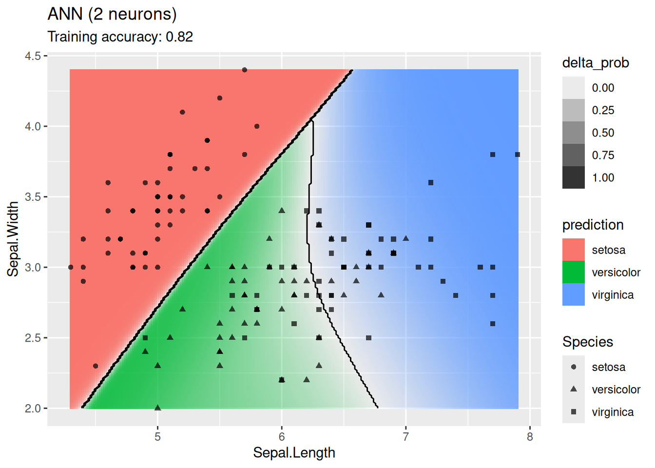
model <- x |> nnet::nnet(Species ~ ., data = _,
                        size = 4, trace = FALSE)
decisionplot(model, x, class_var  = "Species",
             predict_type = c("class", "raw")) +
  labs(title = "ANN (4 neurons)")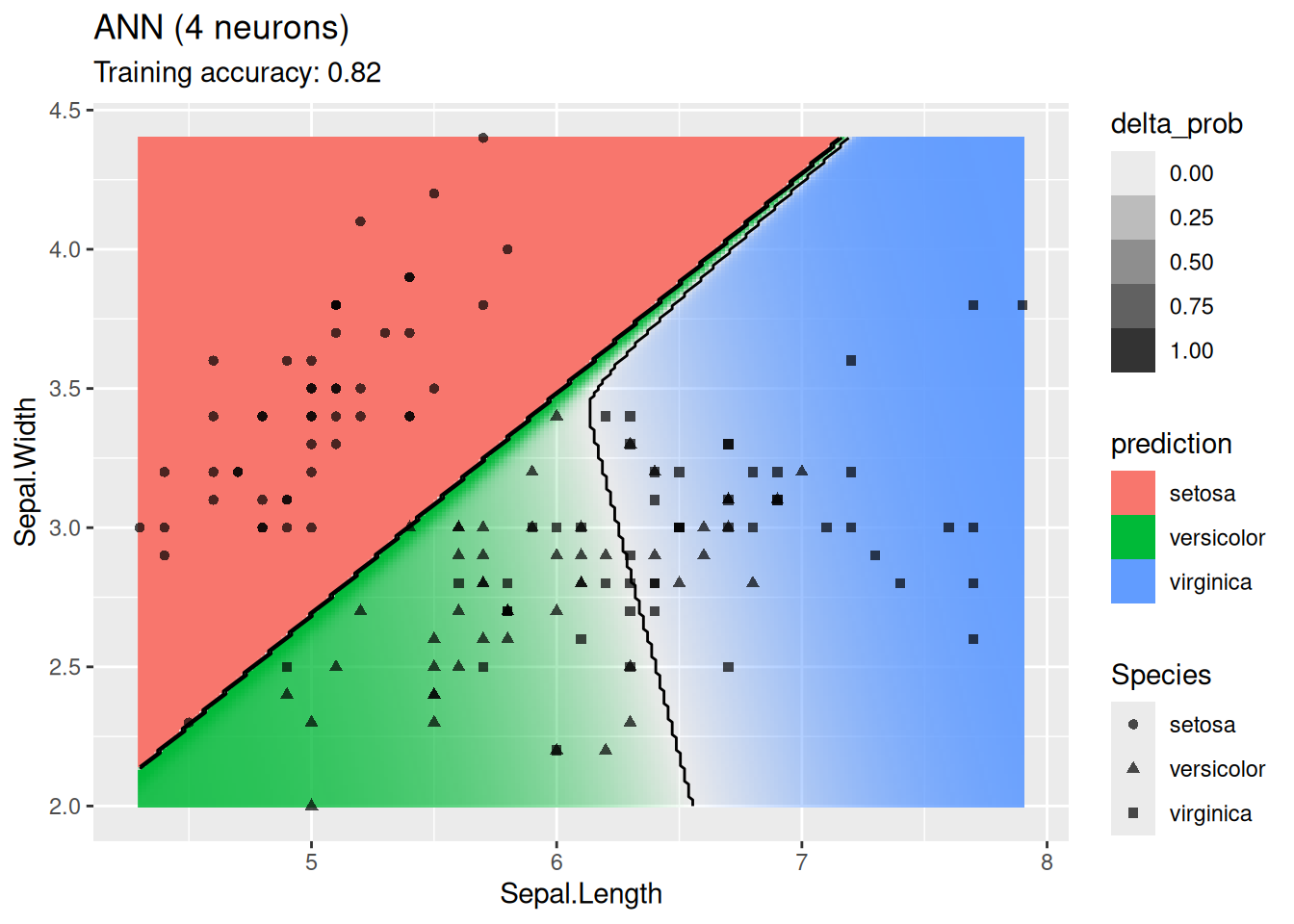
model <- x |> nnet::nnet(Species ~ ., data = _,
                        size = 6, trace = FALSE)
decisionplot(model, x, class_var  = "Species",
             predict_type = c("class", "raw")) +
  labs(title = "ANN (6 neurons)")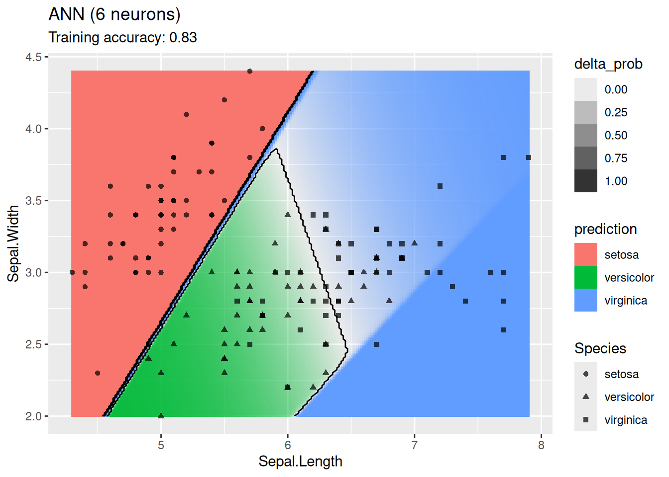
model <- x |> nnet::nnet(Species ~ ., data = _,
                        size = 20, trace = FALSE)
decisionplot(model, x, class_var  = "Species",
             predict_type = c("class", "raw")) +
  labs(title = "ANN (20 neurons)")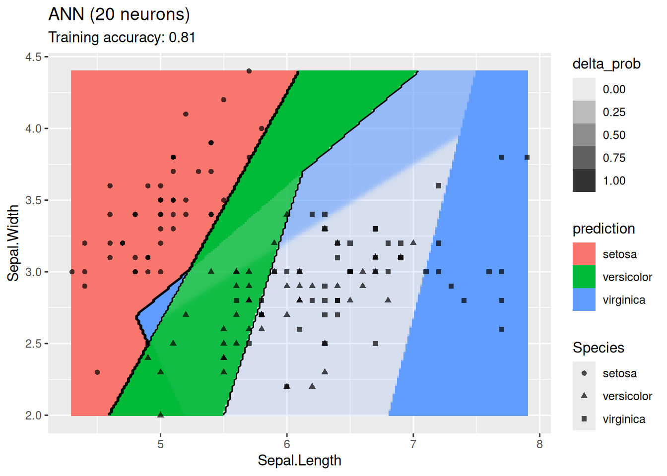
model <- x |> nnet::nnet(Species ~ ., data = _,
                        size = 100, trace = FALSE)
decisionplot(model, x, class_var  = "Species",
             predict_type = c("class", "raw")) +
  labs(title = "ANN (100 neurons)")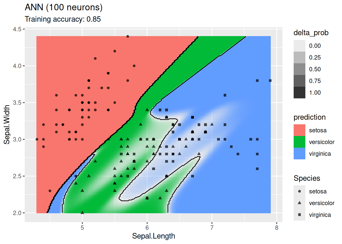
model <- x |> nnet::nnet(Species ~ ., data = _,
                        size = 100, trace = FALSE)
decisionplot(model, x, class_var  = "Species",
             predict_type = c("class", "raw")) +
  labs(title = "ANN 2nd try (100 neurons)")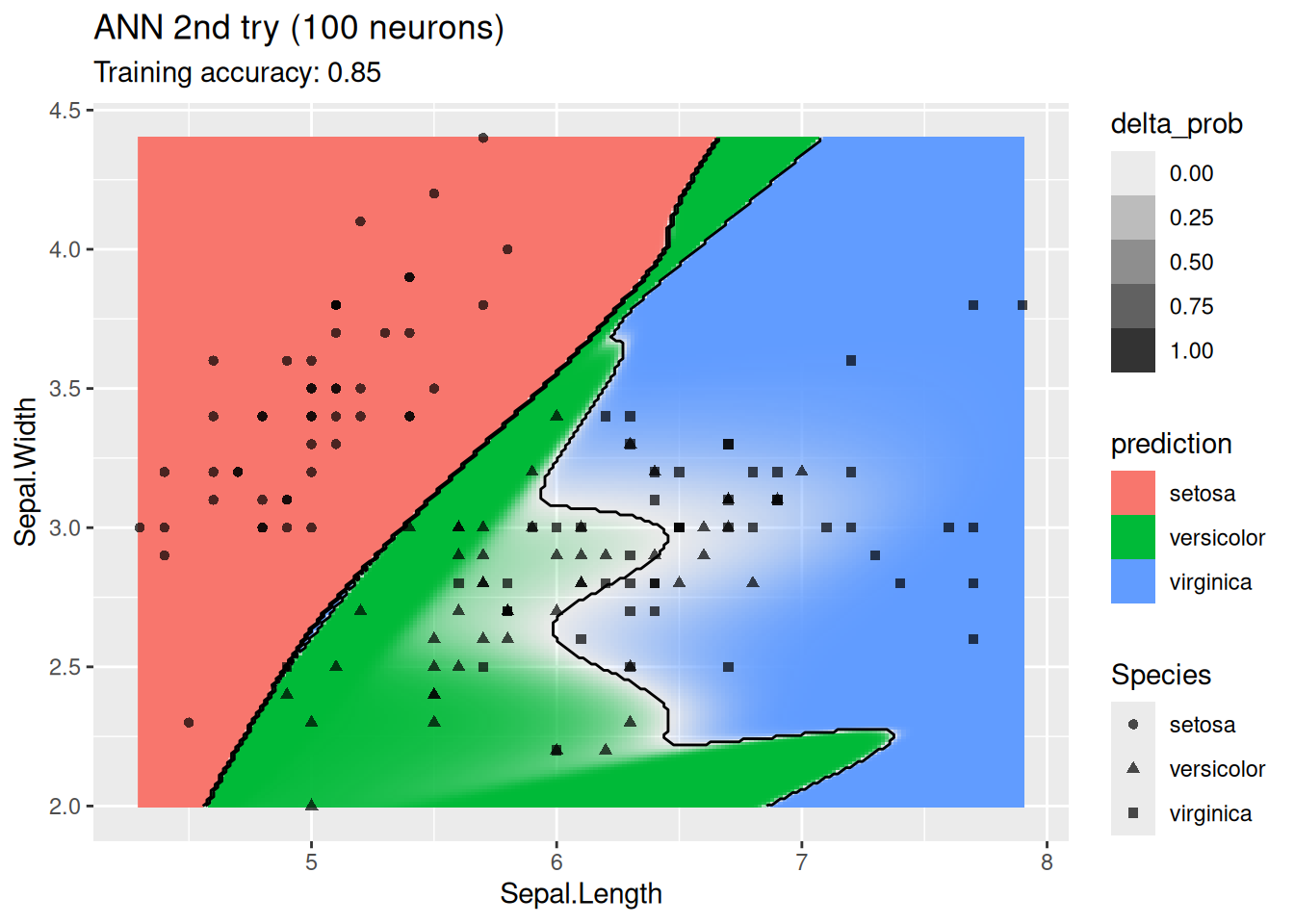
For this simple data set, 2 neurons produce the best classifier. The model starts to overfit with 6 or more neurons. I ran the ANN twice with 100 neurons, the two different decision boundaries indicate that the variability of the ANN with so many neurons is high.
4.14.2 Circle Dataset
set.seed(1000)

x <- mlbench::mlbench.circle(500)

# You can also experiment with the following datasets.
#x <- mlbench::mlbench.cassini(500)
#x <- mlbench::mlbench.spirals(500, sd = .1)
#x <- mlbench::mlbench.smiley(500)

x <- cbind(as.data.frame(x$x), factor(x$classes))
colnames(x) <- c("x", "y", "class")
x <- as_tibble(x)
x
## # A tibble: 500 × 3
##          x       y class
##      <dbl>   <dbl> <fct>
##  1 -0.344   0.448  1
##  2  0.518   0.915  2
##  3 -0.772  -0.0913 1
##  4  0.382   0.412  1
##  5  0.0328  0.438  1
##  6 -0.865  -0.354  2
##  7  0.477   0.640  2
##  8  0.167  -0.809  2
##  9 -0.568  -0.281  1
## 10 -0.488   0.638  2
## # ℹ 490 more rows
ggplot(x, aes(x = x, y = y, color = class)) +
  geom_point()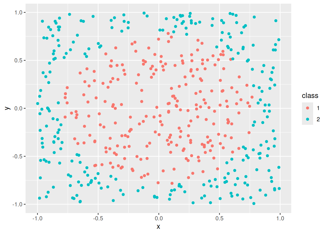
This dataset is challenging for some classification algorithms since the optimal decision boundary is a circle around the class in the center.
4.14.2.1 Nearest Neighbor Classifier
Compare kNN classifiers with different values for \(k\).
model <- x |> caret::knn3(class ~ ., data = _, k = 1)
decisionplot(model, x, class_var = "class") +
  labs(title = "kNN (1 neighbor)")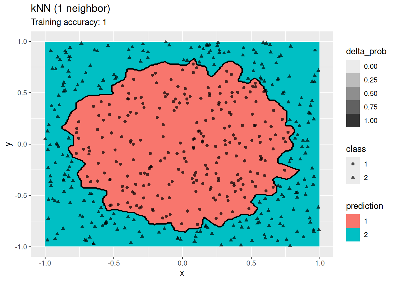
model <- x |> caret::knn3(class ~ ., data = _, k = 10)
decisionplot(model, x, class_var = "class") +
  labs(title = "kNN (10 neighbors)")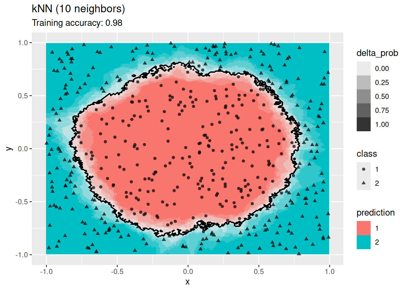
k-Nearest does not find a smooth decision boundary, but tends to overfit the training data at low values for \(k\).
4.14.2.2 Naive Bayes Classifier
The Gaussian naive Bayes classifier works very well on the data.
model <- x |> e1071::naiveBayes(class ~ ., data = _)
decisionplot(model, x, class_var = "class",
  predict_type = c("class", "raw")) +
  labs(title = "naive Bayes")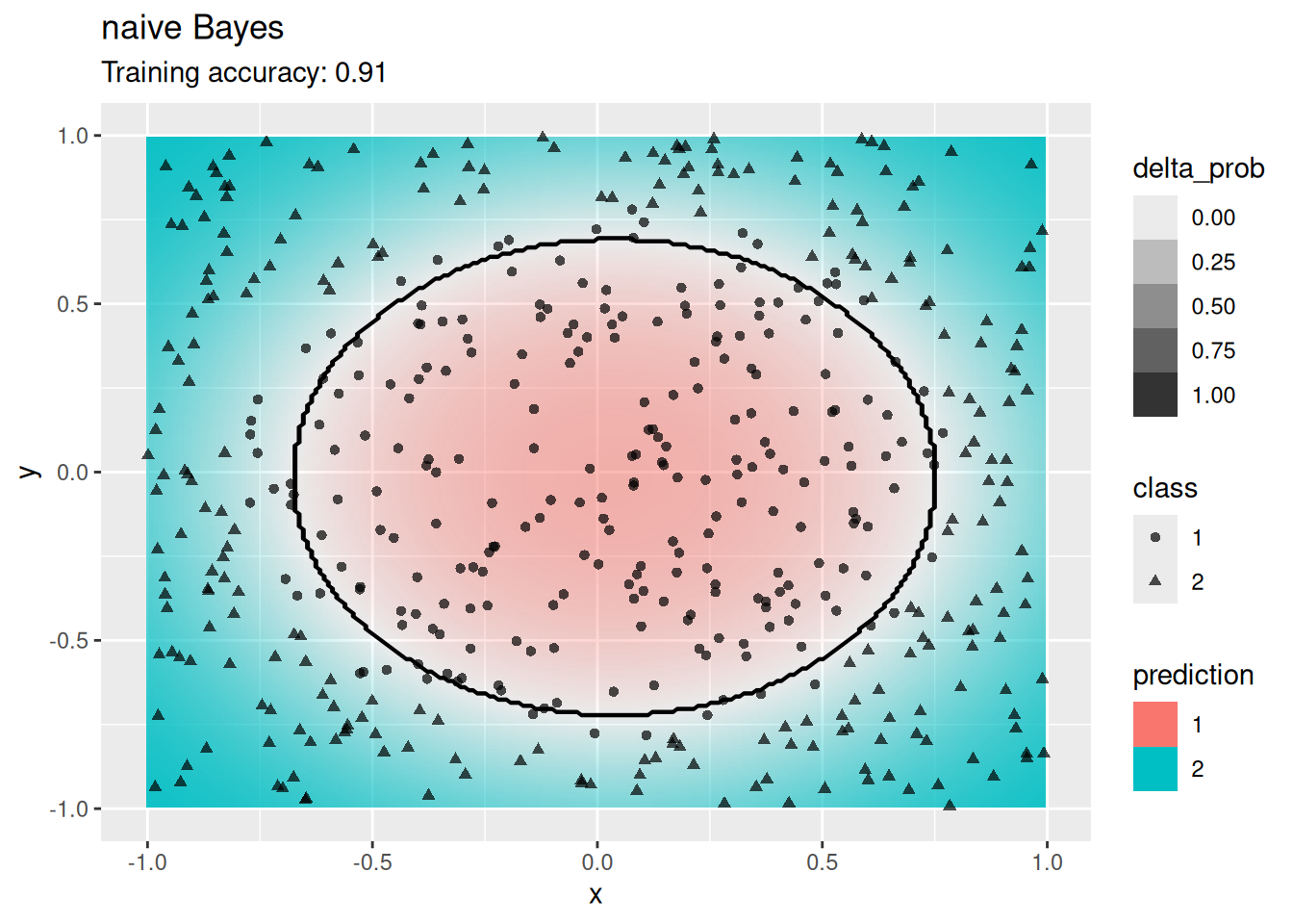
4.14.2.3 Linear Discriminant Analysis
LDA cannot find a good model since the true decision boundary is not linear.
model <- x |> MASS::lda(class ~ ., data = _)
decisionplot(model, x, class_var = "class") + labs(title = "LDA")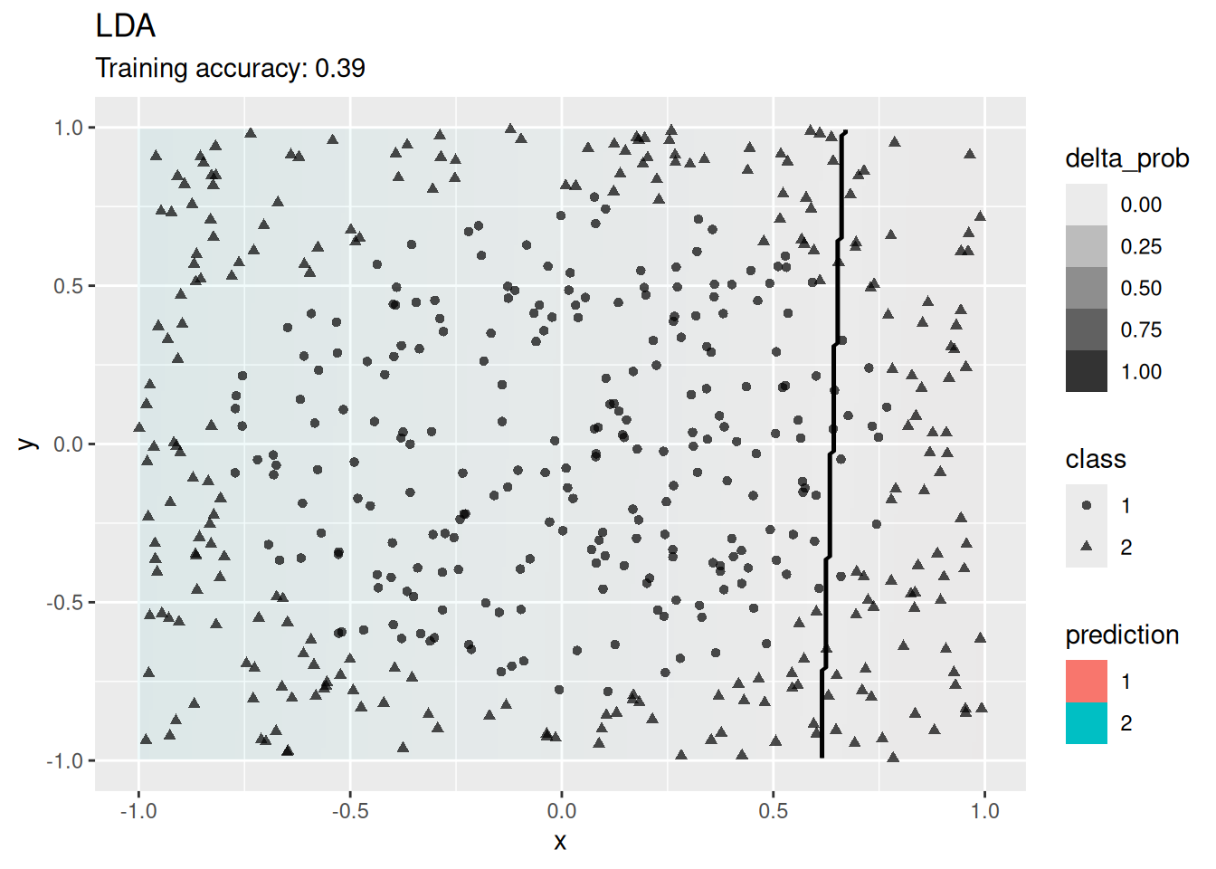
4.14.2.4 Multinomial Logistic Regression
Multinomial logistic regression is an extension of logistic regression to problems with more than two classes.
model <- x |> nnet::multinom(class ~., data = _)
## # weights:  4 (3 variable)
## initial  value 346.573590
## final  value 346.308371
## converged
decisionplot(model, x, class_var = "class") +
  labs(titel = "Multinomial Logistic Regression")
## Ignoring unknown labels:
## • titel : "Multinomial Logistic Regression"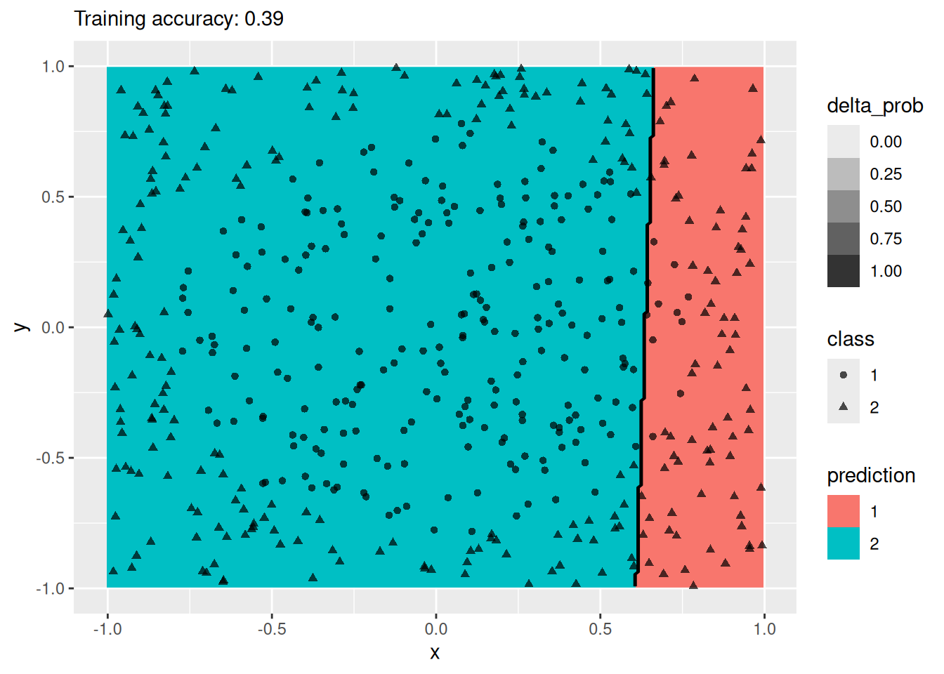
Logistic regression also tries to find a linear decision boundary and fails.
4.14.2.5 Decision Trees
Compare different decision tree algorithms.
model <- x |> rpart::rpart(class ~ ., data = _)
decisionplot(model, x, class_var = "class") +
  labs(title = "CART")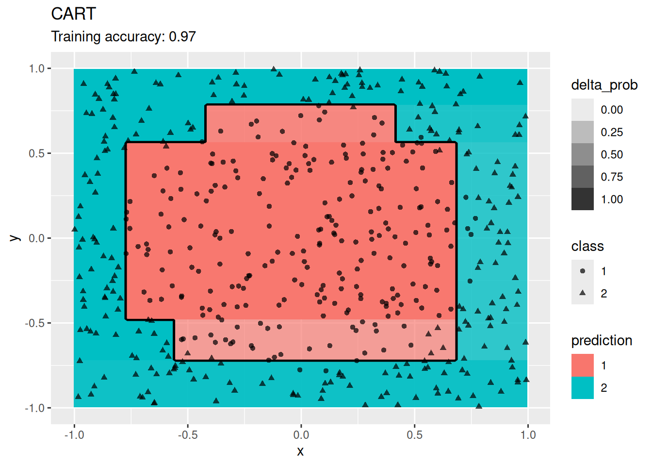
model <- x |> rpart::rpart(class ~ ., data = _,
  control = rpart::rpart.control(cp = 0, minsplit = 1))
decisionplot(model, x, class_var = "class") +
  labs(title = "CART (overfitting)")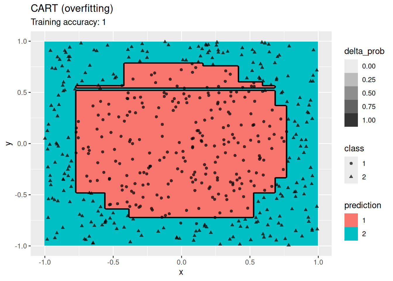
model <- x |> C50::C5.0(class ~ ., data = _)
decisionplot(model, x, class_var = "class") +
  labs(title = "C5.0")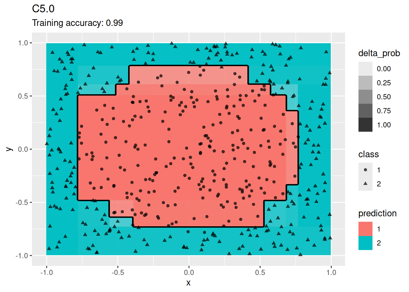
Decision trees do well with the restriction that they can only create cuts parallel to the axes.
4.14.2.6 Ensemble: Random Forest
Try random forest on the dataset.
library(randomForest)
## randomForest 4.7-1.2
## Type rfNews() to see new features/changes/bug fixes.
##
## Attaching package: 'randomForest'
## The following object is masked from 'package:dplyr':
##
##     combine
## The following object is masked from 'package:ggplot2':
##
##     margin
model <- x |> randomForest(class ~ ., data = _)
decisionplot(model, x, class_var = "class") +
  labs(title = "Random Forest")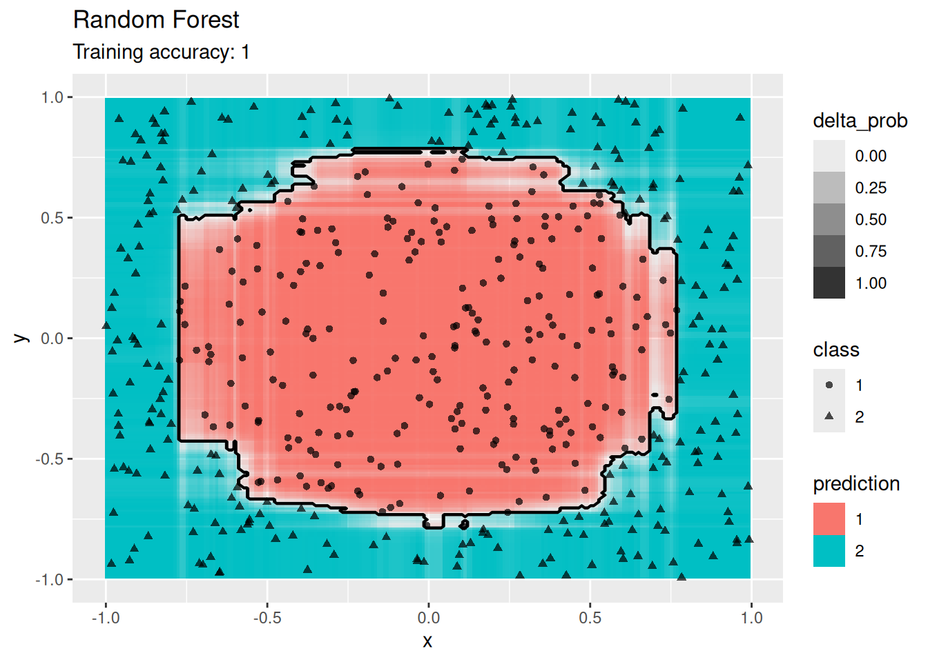
4.14.2.7 Support Vector Machine
Compare SVMs with different kernels.
model <- x |> e1071::svm(class ~ ., data = _,
                         kernel = "linear", probability = TRUE)
decisionplot(model, x, class_var = "class") +
  labs(title = "SVM (linear kernel)")
## Warning: Computation failed in `stat_contour()`.
## Caused by error in `zero_range()`:
## ! `x` must be length 1 or 2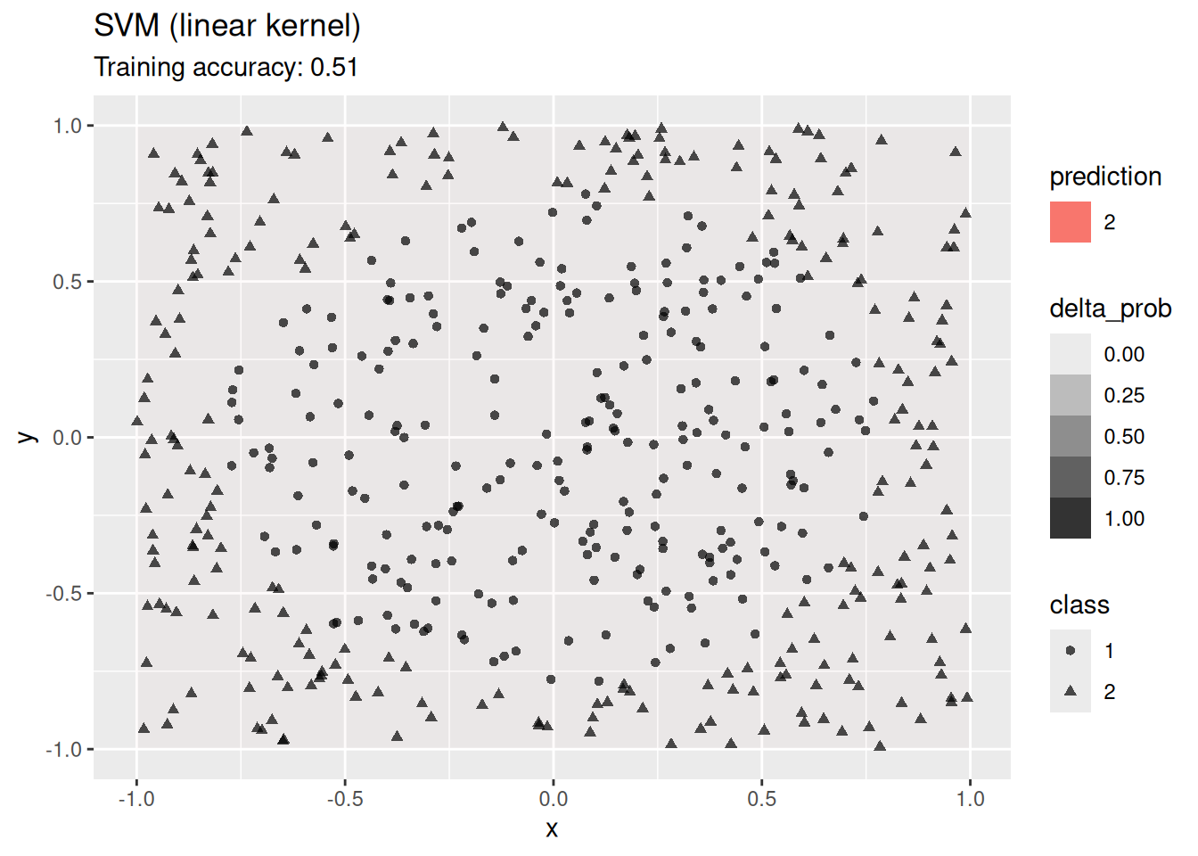
model <- x |> e1071::svm(class ~ ., data = _,
                         kernel = "radial", probability = TRUE)
decisionplot(model, x, class_var = "class") +
  labs(title = "SVM (radial kernel)")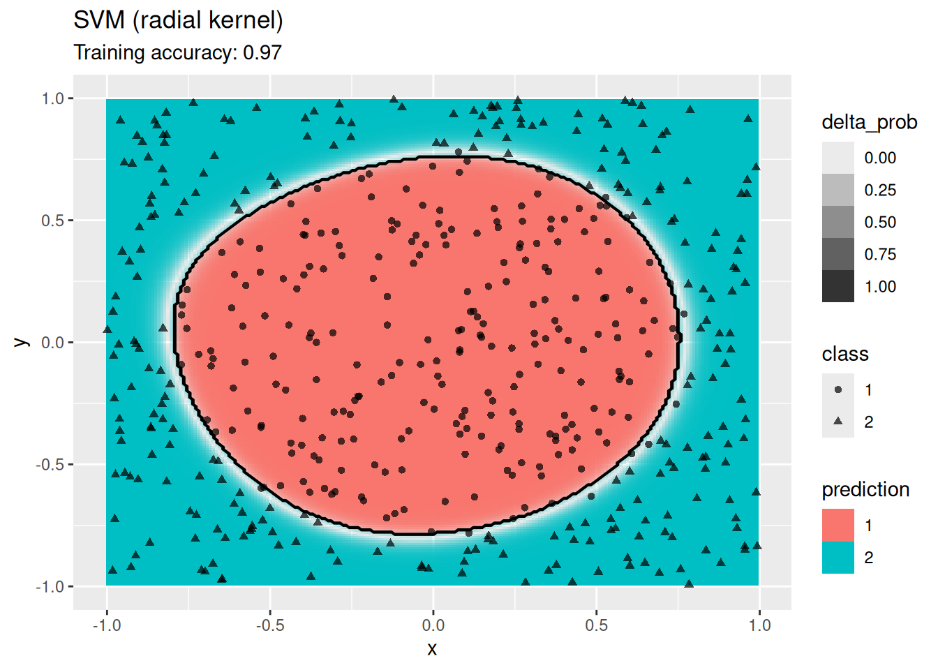
model <- x |> e1071::svm(class ~ ., data = _,
                         kernel = "polynomial", probability = TRUE)
decisionplot(model, x, class_var = "class") +
  labs(title = "SVM (polynomial kernel)")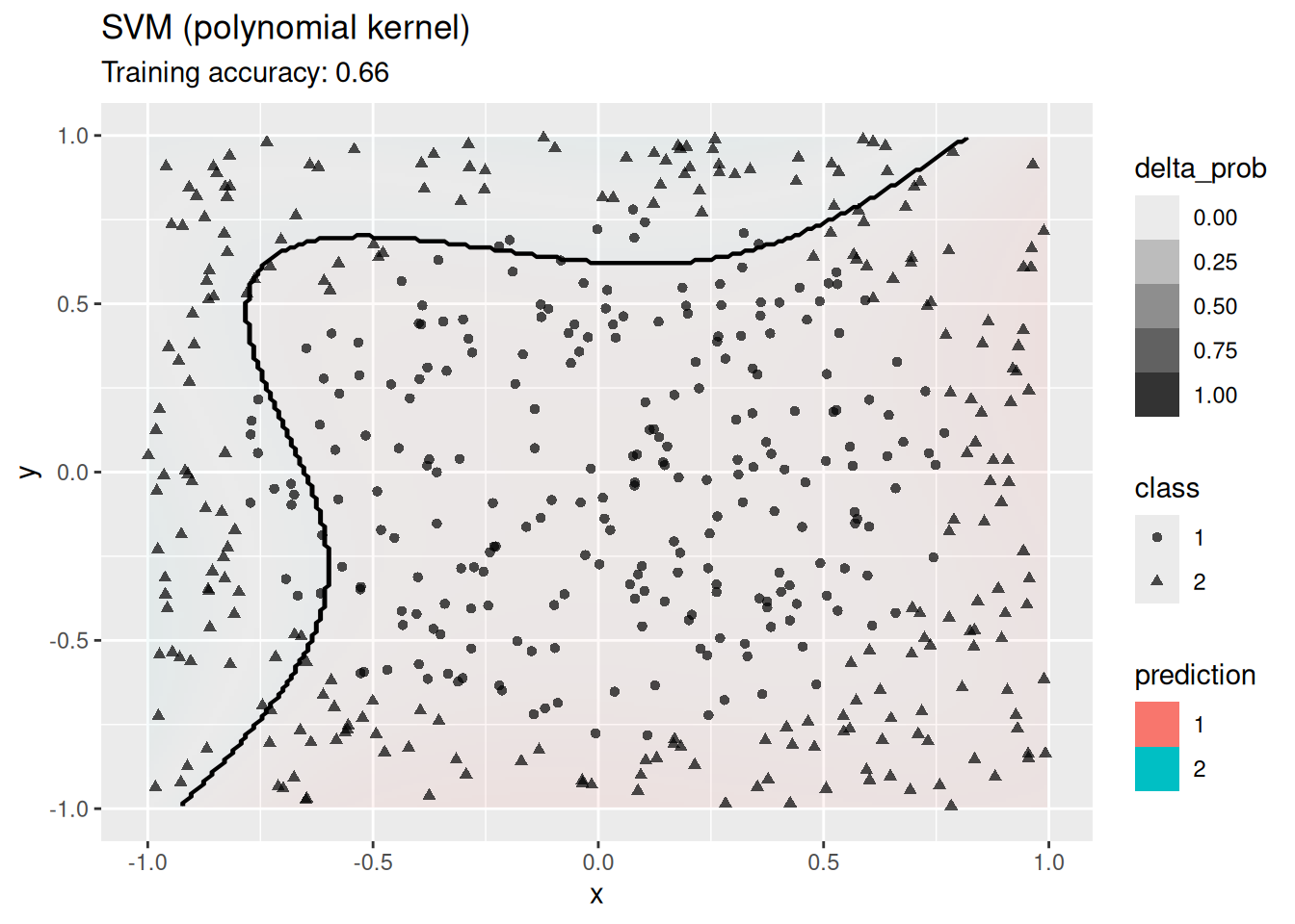
model <- x |> e1071::svm(class ~ ., data = _,
                         kernel = "sigmoid", probability = TRUE)
decisionplot(model, x, class_var = "class") +
  labs(title = "SVM (sigmoid kernel)")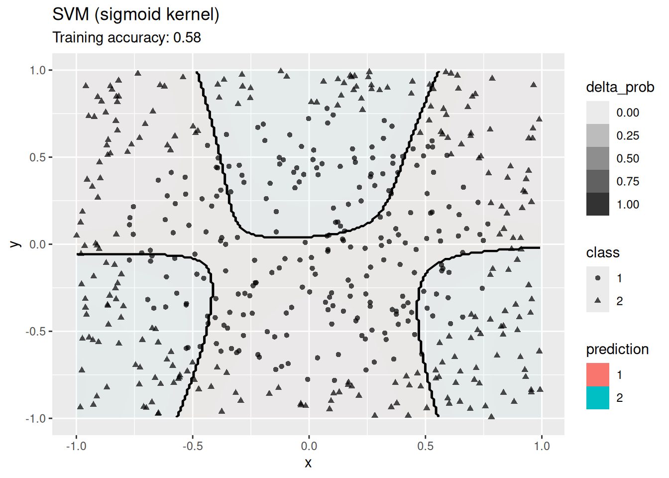
A linear SVM does not work on this data set. An SMV with a radial kernel performs well, the other kernels have issues with finding a linear decision boundary in the projected space.
4.14.2.8 Single Layer Feed-forward Neural Networks
Use a simple network with one hidden layer. We will try a different number of neurons for the hidden layer.
model <- x |> nnet::nnet(class ~ ., data = _, size = 1, trace = FALSE)
decisionplot(model, x, class_var = "class",
  predict_type = c("class", "raw")) + labs(title = "ANN (1 neuron)")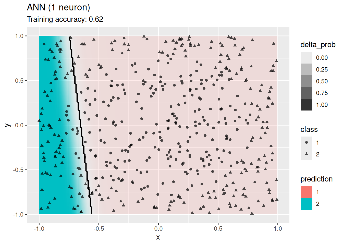
model <- x |> nnet::nnet(class ~ ., data = _, size = 2, trace = FALSE)
decisionplot(model, x, class_var = "class",
  predict_type = c("class", "raw")) + labs(title = "ANN (2 neurons)")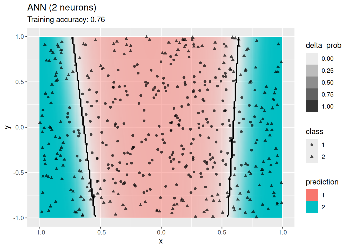
model <- x |> nnet::nnet(class ~ ., data = _, size = 4, trace = FALSE)
decisionplot(model, x, class_var = "class",
  predict_type = c("class", "raw")) + labs(title = "ANN (4 neurons)")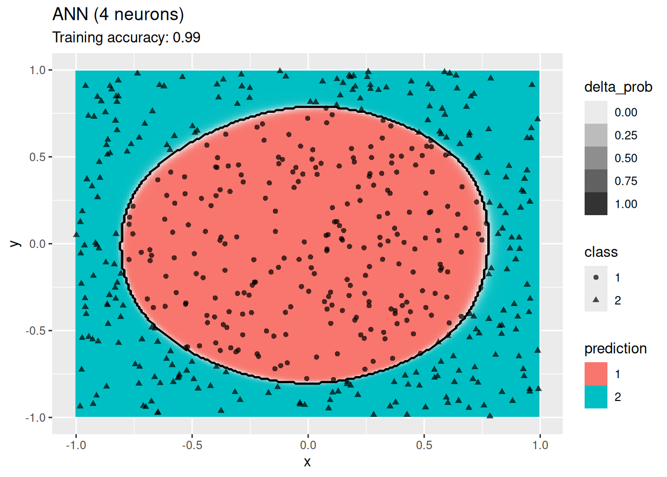
model <- x |> nnet::nnet(class ~ ., data = _, size = 6, trace = FALSE)
decisionplot(model, x, class_var = "class",
  predict_type = c("class", "raw")) + labs(title = "ANN (6 neurons)")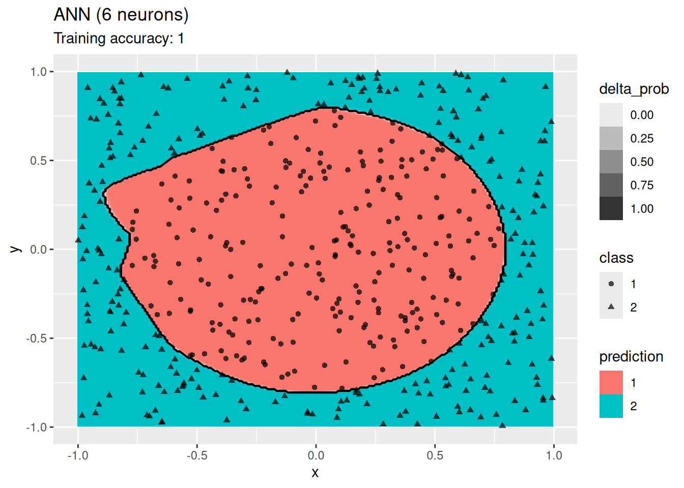
model <- x |> nnet::nnet(class ~ ., data = _, size = 20, trace = FALSE)
decisionplot(model, x, class_var = "class",
  predict_type = c("class", "raw")) + labs(title = "ANN (20 neurons)")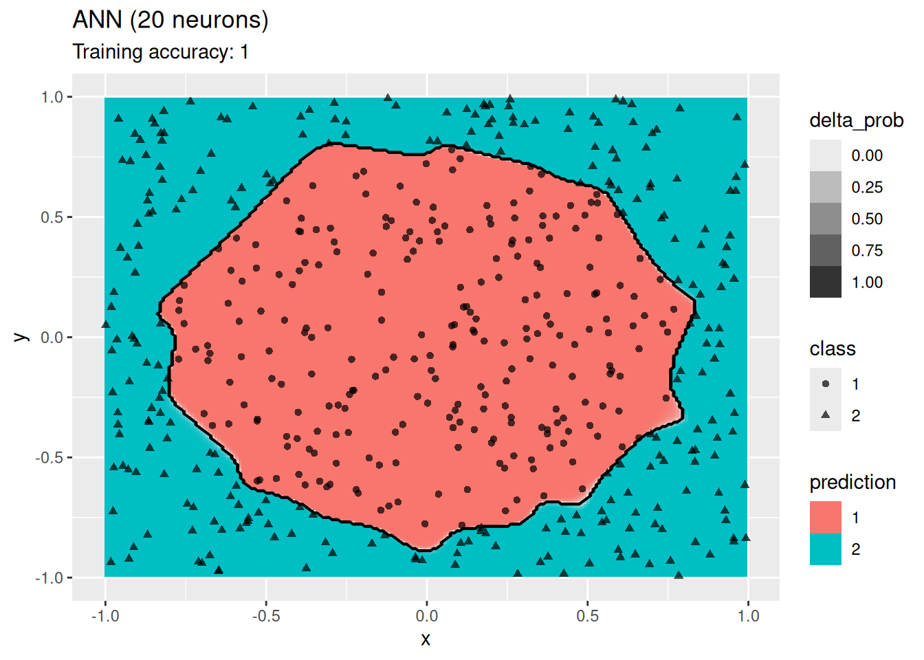
The plots show that a network with 4 and 6 neurons performs well, while a larger number of neurons leads to overfitting the training data.
4.15 More Information on Classification with R
- The
caretframework used in this book: https://topepo.github.io/caret/ - Alternative modeling framework (not used in these examples): https://www.tidymodels.org/
- R taskview on machine learning: http://cran.r-project.org/web/views/MachineLearning.html
4.16 Exercises*
We will again use the Palmer penguin data for the exercises.
library(palmerpenguins)
##
## Attaching package: 'palmerpenguins'
## The following objects are masked from 'package:datasets':
##
##     penguins, penguins_raw
head(penguins)
## # A tibble: 6 × 8
##   species island    bill_length_mm bill_depth_mm
##   <fct>   <fct>              <dbl>         <dbl>
## 1 Adelie  Torgersen           39.1          18.7
## 2 Adelie  Torgersen           39.5          17.4
## 3 Adelie  Torgersen           40.3          18
## 4 Adelie  Torgersen           NA            NA
## 5 Adelie  Torgersen           36.7          19.3
## 6 Adelie  Torgersen           39.3          20.6
## # ℹ 4 more variables: flipper_length_mm <int>,
## #   body_mass_g <int>, sex <fct>, year <int>
Create a R markdown file with the code and do the following below.
- Apply at least 3 different classification models to the data.
- Compare the models and a simple baseline model. Which model performs the best? Does it perform significantly better than the other models?
A good answer should compare at least three classifiers with a simple baseline on the same data split and using the same metrics. Explain how model settings were selected using training data, support the comparison with resampling or test results, and discuss uncertainty. Treat “significantly better” as a statistical claim that needs appropriate evidence, not just a small difference in reported accuracy.
4.17 Chapter Summary
This chapter compares rule-based PART, nearest-neighbor, naive Bayes, Bayesian network, logistic regression, neural network, support vector machine, and ensemble classifiers including random forests. These methods make different assumptions and can produce different decision boundaries, so compare them against a baseline using the same training and test data and suitable metrics. For imbalanced classes, accuracy can hide poor detection of the minority class; options include retaining the original distribution, upsampling within resampling, adjusting probability thresholds, and using cost-sensitive learning. Visualizing boundaries on iris and synthetic circle data helps show how model choices shape predictions.
4.18 Key Terms
- Baseline classifier: a simple reference model used to contextualize performance.
- Class imbalance: a large difference in the number of examples per class.
- Decision boundary: the feature-space boundary separating predicted classes.
- Sensitivity: the fraction of actual positive cases correctly identified.
- Threshold: a probability cutoff used to turn predicted probabilities into class labels.