C Logistic Regression
This chapter examines logistic regression in more detail. Logistic regression is introduced as an alternative classification method in Chapter 4 of Introduction to Data Mining.
C.1 Learning Objectives
After this chapter, you should be able to:
- fit a binary logistic regression model and interpret its coefficients;
- convert model scores into class probabilities and predicted labels;
- assess classification performance on held-out data; and
- recognize when regularized or multinomial logistic regression is appropriate.
C.2 Prerequisites
Read Classification: Basic Concepts and Regression. Familiarity with probability, odds, model formulas, and train/test evaluation is assumed.
pkgs <- c("glmnet", "caret")

pak::pkg_install(pkgs)
The packages used for this chapter are:
- caret (Kuhn 2024)
- glmnet (Friedman et al. 2026)
C.3 Introduction
Despite its name, logistic regression is a classification model for estimating the probability \(p\) of a binary outcome from a set of features. It is a common baseline because it is interpretable and often fits quickly.
Logistic regression is a generalized linear model with the logit link and a binomial response distribution. It models the log odds of the binary outcome as a linear function of the predictors:
\[logit(p) = ln\left(\frac{p}{1-p}\right) = \beta_0 + \beta_1 x_1 + \beta_2 x_2 + ...\]
The logit function maps a probability \(p\) in \((0,1)\) to the real line \((-\infty,+\infty)\).
logit  <- function(p) log(p/(1-p))
p <- seq(0, 1, length.out = 100)
plot(logit(p), p, type = "l")
abline(h = 0.5, lty = 2)
abline(v = 0, lty = 2)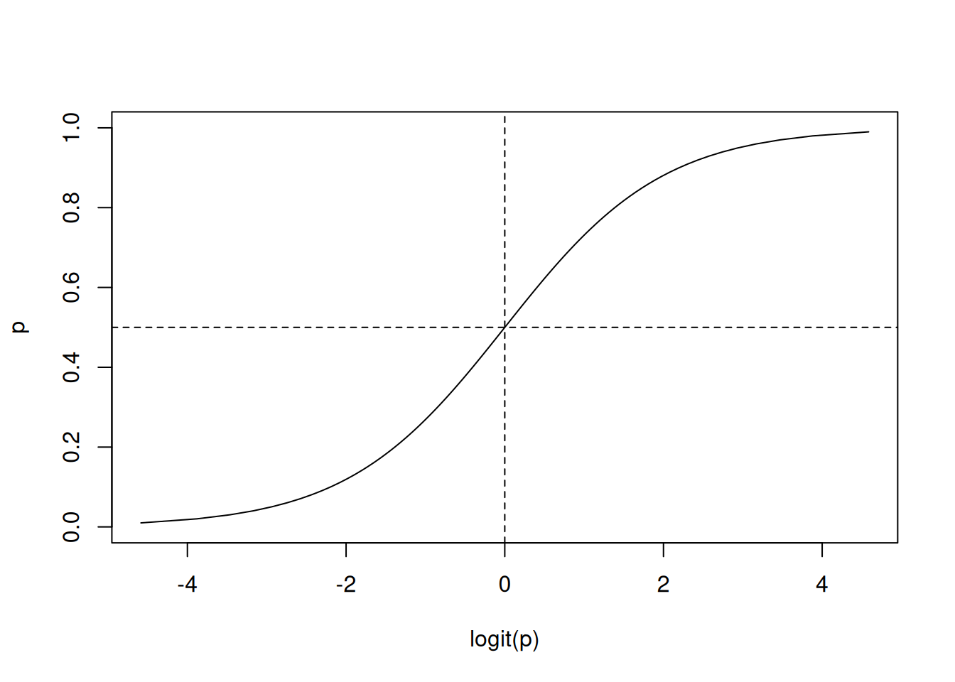
The plotted curve is the inverse logit, also called the logistic or sigmoid function. It maps real-valued linear predictors to probabilities in \((0,1)\). Using the inverse function, we see that the probability of the outcome \(p\) is modeled by the logistic function of the linear regression:
\[ p = \frac{e^{\beta_0 + \beta_1 x_1 + \beta_2 x_2 + ...}}{1 + e^{\beta_0 + \beta_1 x_1 + \beta_2 x_2 + ...}} = \frac{1}{1+e^{-(\beta_0 + \beta_1 x_1 + \beta_2 x_2 + ...)}} = \sigma(\beta_0 + \beta_1 x_1 + \beta_2 x_2 + ...)\]
After estimating \(\boldsymbol{\beta} = (\beta_0, \beta_1,...)\) from training data by maximizing the binomial likelihood (equivalently, minimizing log loss), the equation above predicts the probability \(p\) for a new data point \(\mathbf{x} = (x_1, x_2, ...)\). With a default threshold of 0.5, we predict the event when \(p > .5\) and otherwise predict that it does not occur.
Each binary outcome is modeled with a Bernoulli distribution. Across multiple observations, the number of positive outcomes has a binomial distribution. Logistic regression uses the logit link to relate the event probability to the linear predictor.
C.4 Data Preparation
We load and shuffle the data. We also add a useless variable to see if the logistic regression removes it.
data(iris)
set.seed(100) # for reproducibility

x <- iris[sample(1:nrow(iris)),]
x <- cbind(x, useless = rnorm(nrow(x)))
We create a binary classification problem by
asking if a flower is of species Virginica or not.
We create new logical variable called virginica and remove the
Species column.
x$virginica <- x$Species == "virginica"
x$Species <- NULL
We can visualize the data using a scatter plot matrix and use the color red for
virginica == TRUE and black for the other flowers.
plot(x, col=x$virginica + 1)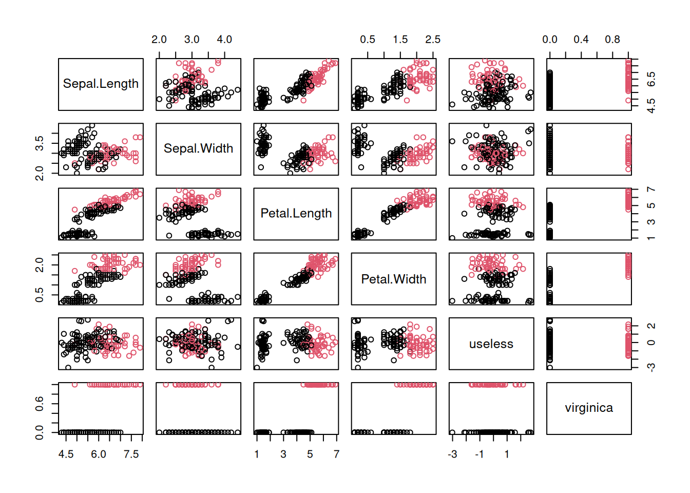
C.5 A first Logistic Regression Model
Logistic regression is a generalized linear model (GLM) with logit as the
link function and a binomial distribution. The glm() function is provided by
the R core package stats which is installed with R and automatically loads
when R is started.
model <- glm(virginica ~ .,
  family = binomial(logit), data = x)
## Warning: glm.fit: fitted probabilities numerically 0 or 1
## occurred
About the warning: glm.fit: fitted probabilities numerically 0 or 1 occurred means that the data is possibly linearly separable.
model
##
## Call:  glm(formula = virginica ~ ., family = binomial(logit), data = x)
##
## Coefficients:
##  (Intercept)  Sepal.Length   Sepal.Width  Petal.Length
##      -41.649        -2.531        -6.448         9.376
##  Petal.Width       useless
##       17.696         0.098
##
## Degrees of Freedom: 149 Total (i.e. Null);  144 Residual
## Null Deviance:       191
## Residual Deviance: 11.9  AIC: 23.9
Check which features are significant?
summary(model)
##
## Call:
## glm(formula = virginica ~ ., family = binomial(logit), data = x)
##
## Coefficients:
##              Estimate Std. Error z value Pr(>|z|)
## (Intercept)   -41.649     26.556   -1.57    0.117
## Sepal.Length   -2.531      2.458   -1.03    0.303
## Sepal.Width    -6.448      4.794   -1.34    0.179
## Petal.Length    9.376      4.763    1.97    0.049 *
## Petal.Width    17.696     10.632    1.66    0.096 .
## useless         0.098      0.807    0.12    0.903
## ---
## Signif. codes:
## 0 '***' 0.001 '**' 0.01 '*' 0.05 '.' 0.1 ' ' 1
##
## (Dispersion parameter for binomial family taken to be 1)
##
##     Null deviance: 190.954  on 149  degrees of freedom
## Residual deviance:  11.884  on 144  degrees of freedom
## AIC: 23.88
##
## Number of Fisher Scoring iterations: 12
AIC (Akaike information criterion) is a measure of how good the model is. Smaller is better. It can be used for model selection.
The parameter estimates in the coefficients table are log odds. The * and .
indicate if the effect of the parameter is significantly different from 0.
Positive numbers
mean that increasing the variable increases the predicted probability
and negative numbers mean that the probability decreases. For example,
observing a larger Petal.Length increases the predicted probability for the flower to
be of class Virginica. This effect is significant and you can
verify it in the scatter plot above. For Petal.Length, the red dots have
larger values than
the black dots.
C.6 Stepwise Variable Selection
Only two variables were flagged as significant. We can remove insignificant
variables by trying to remove one variable at a time
as long as the model does not significantly deteriorate (according to the AIC).
This variable selection process is done automatically by the step() function.
model2 <- step(model, data = x)
## Start:  AIC=23.88
## virginica ~ Sepal.Length + Sepal.Width + Petal.Length + Petal.Width +
##     useless
## Warning: glm.fit: fitted probabilities numerically 0 or 1
## occurred
## Warning: glm.fit: fitted probabilities numerically 0 or 1
## occurred
## Warning: glm.fit: fitted probabilities numerically 0 or 1
## occurred
## Warning: glm.fit: fitted probabilities numerically 0 or 1
## occurred
## Warning: glm.fit: fitted probabilities numerically 0 or 1
## occurred
##                Df Deviance  AIC
## - useless       1     11.9 21.9
## - Sepal.Length  1     13.2 23.2
## <none>                11.9 23.9
## - Sepal.Width   1     14.8 24.8
## - Petal.Width   1     22.4 32.4
## - Petal.Length  1     25.9 35.9
## Warning: glm.fit: fitted probabilities numerically 0 or 1
## occurred
##
## Step:  AIC=21.9
## virginica ~ Sepal.Length + Sepal.Width + Petal.Length + Petal.Width
## Warning: glm.fit: fitted probabilities numerically 0 or 1
## occurred
## Warning: glm.fit: fitted probabilities numerically 0 or 1
## occurred
## Warning: glm.fit: fitted probabilities numerically 0 or 1
## occurred
## Warning: glm.fit: fitted probabilities numerically 0 or 1
## occurred
##                Df Deviance  AIC
## - Sepal.Length  1     13.3 21.3
## <none>                11.9 21.9
## - Sepal.Width   1     15.5 23.5
## - Petal.Width   1     23.8 31.8
## - Petal.Length  1     25.9 33.9
## Warning: glm.fit: fitted probabilities numerically 0 or 1
## occurred
##
## Step:  AIC=21.27
## virginica ~ Sepal.Width + Petal.Length + Petal.Width
## Warning: glm.fit: fitted probabilities numerically 0 or 1
## occurred
## Warning: glm.fit: fitted probabilities numerically 0 or 1
## occurred
##                Df Deviance  AIC
## <none>                13.3 21.3
## - Sepal.Width   1     20.6 26.6
## - Petal.Length  1     27.4 33.4
## - Petal.Width   1     31.5 37.5
summary(model2)
##
## Call:
## glm(formula = virginica ~ Sepal.Width + Petal.Length + Petal.Width,
##     family = binomial(logit), data = x)
##
## Coefficients:
##              Estimate Std. Error z value Pr(>|z|)
## (Intercept)    -50.53      23.99   -2.11    0.035 *
## Sepal.Width     -8.38       4.76   -1.76    0.079 .
## Petal.Length     7.87       3.84    2.05    0.040 *
## Petal.Width     21.43      10.71    2.00    0.045 *
## ---
## Signif. codes:
## 0 '***' 0.001 '**' 0.01 '*' 0.05 '.' 0.1 ' ' 1
##
## (Dispersion parameter for binomial family taken to be 1)
##
##     Null deviance: 190.954  on 149  degrees of freedom
## Residual deviance:  13.266  on 146  degrees of freedom
## AIC: 21.27
##
## Number of Fisher Scoring iterations: 12
The estimates (\(\beta_0, \beta_1,...\) ) are log-odds and can be converted into odds using \(exp(\beta)\). A negative log-odds ratio means that the odds go down with an increase in the value of the predictor. A predictor with a positive log-odds ratio increases the odds. In this case, the odds of looking at a Virginica iris goes down with Sepal.Width and increases with the other two predictors.
C.7 Calculate the Response
Note: we do here in-sample testing on the data we learned the data from. To get a generalization error estimate you should use a test set or cross-validation!
pr <- predict(model2, x, type = "response")
round(pr[1:10], 2)
##  102  112    4   55   70   98  135    7   43  140
## 1.00 1.00 0.00 0.00 0.00 0.00 0.86 0.00 0.00 1.00
The response is the predicted probability of the flower being of species Virginica. The probabilities of the first 10 flowers are shown. Below is a histogram of predicted probabilities. The color is used to show the examples that have the true class Virginica.
hist(pr, breaks = 20, main = "Predicted Probability vs. True Class")
hist(pr[x$virginica == TRUE], col = "red", breaks = 20, add = TRUE)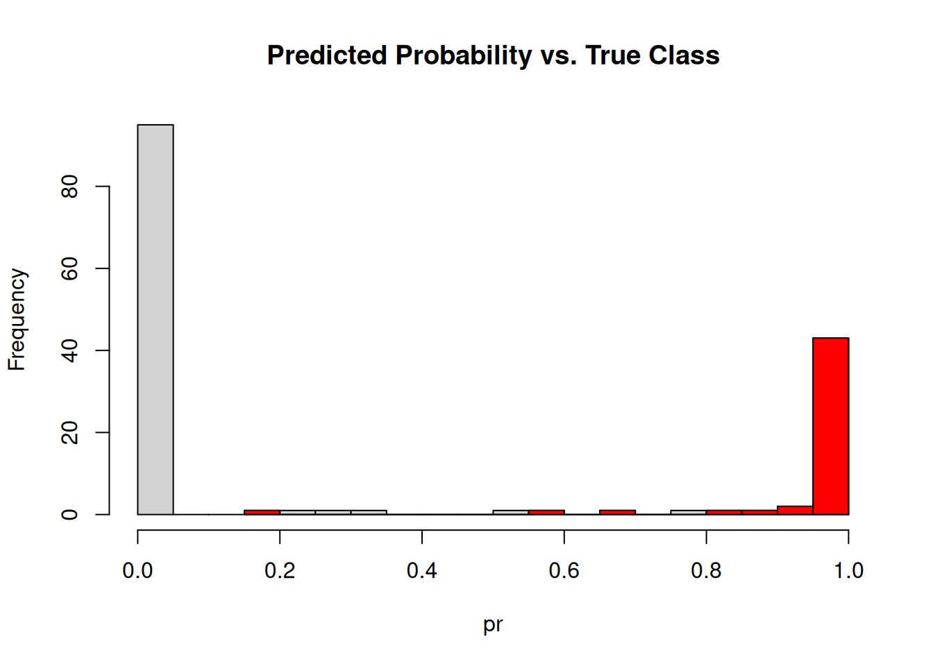
C.8 Illustrate In-Sample Classification Performance
Here we perform in-sample evaluation on the training set. To get an estimate for generalization error, we should calculate the performance on a held out test set.
The predicted class is calculated by checking if the predicted probability is larger than .5.
pred <- pr > .5Now we can create a confusion table and calculate the accuracy.
tbl <- table(predicted = pred, actual = x$virginica)
tbl
##          actual
## predicted FALSE TRUE
##     FALSE    98    1
##     TRUE      2   49
sum(diag(tbl))/sum(tbl)
## [1] 0.98
We can also use caret’s more advanced function caret::confusionMatrix(). Our code
above uses logical vectors. For caret, we need to make sure that both,
the reference and the predictions are coded as factor.
caret::confusionMatrix(
  reference = factor(x$virginica, labels = c("Yes", "No"), levels = c(TRUE, FALSE)),
  data = factor(pred, labels = c("Yes", "No"), levels = c(TRUE, FALSE)))
## Confusion Matrix and Statistics
##
##           Reference
## Prediction Yes No
##        Yes  49  2
##        No    1 98
##
##                Accuracy : 0.98
##                  95% CI : (0.943, 0.996)
##     No Information Rate : 0.667
##     P-Value [Acc > NIR] : <2e-16
##
##                   Kappa : 0.955
##
##  Mcnemar's Test P-Value : 1
##
##             Sensitivity : 0.980
##             Specificity : 0.980
##          Pos Pred Value : 0.961
##          Neg Pred Value : 0.990
##              Prevalence : 0.333
##          Detection Rate : 0.327
##    Detection Prevalence : 0.340
##       Balanced Accuracy : 0.980
##
##        'Positive' Class : Yes
##
These in-sample accuracy and kappa values describe performance on the data used to fit the model and are likely optimistic. Use the held-out test set, as discussed in the previous chapter, to estimate performance on new observations.
C.9 Regularized Logistic Regression
glmnet::glmnet() fits generalized linear models (including logistic regression)
using regularization via penalized maximum likelihood.
The regularization parameter \(\lambda\) is a hyperparameter and
glmnet can use cross-validation to find an appropriate
value. glmnet does not have a function interface, so we have
to supply a matrix for X and a vector of responses for y.
library(glmnet)
## Loading required package: Matrix
## Loaded glmnet 5.1
X <- as.matrix(x[, 1:5])
y <- x$virginica

fit <- cv.glmnet(X, y, family = "binomial")
fit
##
## Call:  cv.glmnet(x = X, y = y, family = "binomial")
##
## Measure: Binomial Deviance
##
##      Lambda Index Measure     SE Nonzero
## min 0.00164    59   0.126 0.0456       5
## 1se 0.00664    44   0.167 0.0422       3
There are several selection rules for lambda, we look at the coefficients of the logistic regression using the lambda that gives the most regularized model such that the cross-validated error is within one standard error of the minimum cross-validated error.
coef(fit, s = fit$lambda.1se)
## 6 x 1 sparse Matrix of class "dgCMatrix"
##              s=0.00664
## (Intercept)    -16.961
## Sepal.Length     .
## Sepal.Width     -1.766
## Petal.Length     2.197
## Petal.Width      6.820
## useless          .
A dot means 0. We see that the predictors Sepal.Length and useless are not used in the prediction giving a models similar to stepwise variable selection above.
A predict function is provided. We need to specify what regularization to use and that we want to predict a class label.
predict(fit, newx = X[1:5,], s = fit$lambda.1se, type = "class")
##     s=0.00664
## 102 "TRUE"
## 112 "TRUE"
## 4   "FALSE"
## 55  "FALSE"
## 70  "FALSE"
Glmnet provides supports many types of generalized linear models. Examples can be found in the article An Introduction to glmnet.
C.10 Multinomial Logistic Regression
Regular logistic regression predicts only one outcome of a binary event represented
by two classes. Extending this model to data with more than two classes
is called multinomial logistic regression,
(or log-linear model).
A popular implementation uses simple artificial neural networks.
Regular logistic regression is equivalent to a single neuron with a
sigmoid (i.e., logistic) activation function optimized with cross-entropy loss.
For multinomial logistic regression, one neuron is used for each class and the
probability distribution is calculated with the softmax activation.
This extension is implemented in nnet::multinom().
set.seed(100)
x <- iris[sample(1:nrow(iris)), ]

model <- nnet::multinom(Species ~., data = x)
## # weights:  18 (10 variable)
## initial  value 164.791843
## iter  10 value 16.177348
## iter  20 value 7.111438
## iter  30 value 6.182999
## iter  40 value 5.984028
## iter  50 value 5.961278
## iter  60 value 5.954900
## iter  70 value 5.951851
## iter  80 value 5.950343
## iter  90 value 5.949904
## iter 100 value 5.949867
## final  value 5.949867
## stopped after 100 iterations
model
## Call:
## nnet::multinom(formula = Species ~ ., data = x)
##
## Coefficients:
##            (Intercept) Sepal.Length Sepal.Width
## versicolor       18.69       -5.458      -8.707
## virginica       -23.84       -7.924     -15.371
##            Petal.Length Petal.Width
## versicolor        14.24      -3.098
## virginica         23.66      15.135
##
## Residual Deviance: 11.9
## AIC: 31.9
We get a \(\boldsymbol{\beta}\) vector with weights for two of the three classes. The third class is used as the default class with all weights set to 0. This can be interpreted as comparing the log odds of each of the two classes with the default class. A positive number means that increasing the variable makes the class more likely and a negative number means the opposite.
Predict the class for the first 5 flowers in the training data.
x[1:5, ]
##     Sepal.Length Sepal.Width Petal.Length Petal.Width
## 102          5.8         2.7          5.1         1.9
## 112          6.4         2.7          5.3         1.9
## 4            4.6         3.1          1.5         0.2
## 55           6.5         2.8          4.6         1.5
## 70           5.6         2.5          3.9         1.1
##        Species
## 102  virginica
## 112  virginica
## 4       setosa
## 55  versicolor
## 70  versicolor
predict(model, x[1:5,])
## [1] virginica  virginica  setosa     versicolor versicolor
## Levels: setosa versicolor virginica
The package glmnet implements also multinomial logistic regression using
glmnet(..., family = "multinomial").
C.11 Exercises
We will again use the Palmer penguin data for the exercises.
library(palmerpenguins)
##
## Attaching package: 'palmerpenguins'
## The following objects are masked from 'package:datasets':
##
##     penguins, penguins_raw
head(penguins)
## # A tibble: 6 × 8
##   species island    bill_length_mm bill_depth_mm
##   <fct>   <fct>              <dbl>         <dbl>
## 1 Adelie  Torgersen           39.1          18.7
## 2 Adelie  Torgersen           39.5          17.4
## 3 Adelie  Torgersen           40.3          18
## 4 Adelie  Torgersen           NA            NA
## 5 Adelie  Torgersen           36.7          19.3
## 6 Adelie  Torgersen           39.3          20.6
## # ℹ 4 more variables: flipper_length_mm <int>,
## #   body_mass_g <int>, sex <fct>, year <int>
Create an R markdown document that performs the following:
- Create a test and a training data set (see section Holdout Method in Chapter 3).
- Create a logistic regression using the training set to predict the variable sex.
- Use stepwise variable selection. What variables are selected?
- What do the parameters for for each of the selected features tell you?
- Predict the sex of the penguins in the test set. Create a confusion table and calculate the accuracy and discuss how well the model works.
A good answer should state how the training and test sets were formed and keep variable selection within the training data. Identify the selected predictors and interpret their coefficients with the outcome coding and reference levels made clear. Use the test confusion table to discuss both correct and incorrect predictions; interpret accuracy in light of the class distribution.
C.12 Chapter Summary
Logistic regression models the probability of a categorical response using a linear predictor and a link function. After preparing data and fitting a binary model, interpret coefficients on the log-odds scale and use predicted probabilities to classify cases at a chosen threshold. In-sample performance illustrates how predictions compare with observed labels, but held-out evaluation is needed to estimate generalization. Stepwise selection provides one approach to choosing predictors, while regularized logistic regression can stabilize models with many or correlated predictors. Multinomial logistic regression extends the method to outcomes with more than two classes.
C.13 Key Terms
- Logit: the logarithm of the odds of an event.
- Odds: the probability of an event divided by the probability it does not occur.
- Logistic function: a transformation that maps a real-valued score to a probability between 0 and 1.
- Odds ratio: the multiplicative change in odds associated with a one-unit predictor change, holding other terms fixed.
- Regularization: a penalty on coefficient size used to improve stability and reduce overfitting.