B Regression
Regression is an important statistical method that is covered the freely available Appendix D of the data mining textbook.
In this extra chapter, we introduce the regression problem and multiple linear regression. In addition, alternative models like regression trees and regularized regression are discussed.
B.1 Learning Objectives
After this chapter, you should be able to:
- fit and interpret a multiple linear regression model;
- compare nested models and assess interactions and categorical predictors;
- generate predictions and explain their uncertainty and limitations; and
- compare linear regression with tree-based and regularized alternatives.
B.2 Prerequisites
Read Classification: Basic Concepts for the train/test distinction. Basic knowledge of descriptive statistics, correlation, and algebra is assumed.
Packages Used in this Chapter
pkgs <- c('lars', 'rpart', 'rpart.plot', 'nnet', 'tidyverse')

pak::pkg_install(pkgs)
The packages used for this chapter are:
- lars (Hastie and Efron 2022)
- nnet (B. Ripley 2026)
- rpart (Therneau and Atkinson 2026)
- rpart.plot (Milborrow 2026)
- tidyverse (Wickham 2023)
B.3 Introduction
Recall that classification predicts one of a small set of discrete (i.e., nominal) labels (e.g., yes or no, small, medium or large). Regression is also a supervised learning problem, but its goal is to predict a numeric response from a set of predictors. We start with the popular linear regression and will later discuss alternative regression methods.
Linear regression models a response \(y\) as a linear function of predictors \(X_1, X_2, ..., X_p\) (also called explanatory variables or covariates). With multiple predictors, the model is called multiple linear regression. The linear regression model is: \[y_i = \beta_0 + \beta_1 x_{i1} + \dots + \beta_p x_{ip} + \epsilon_i, \qquad \hat{y}_i = \beta_0 + \beta_1 x_{i1} + \dots + \beta_p x_{ip},\]
where \(\beta_0\) is the intercept, \(\boldsymbol{\beta}\) is a \(p+1\)-dimensional parameter vector learned from the data, and \(\epsilon_i\) is the random error term. The observed residual is \(e_i = y_i - \hat{y}_i\). In vector notation, the model is \[\mathbf{y} = \mathbf{X} \boldsymbol{\beta} + \boldsymbol{\epsilon},\] and its fitted values are \[\hat{\mathbf{y}} = \mathbf{X} \boldsymbol{\beta}.\] Here, \(\mathbf{X}\) is the design matrix containing the predictors.
The error that is often minimized in regression problems is the squared error defined as:
\[SE= \sum_i (y_i - f(\mathbf{x}_i))^2\]
The parameter vector is estimated by minimizing the sum of squared residuals in the training data.
Linear regression makes several assumptions that should be checked:
- Linearity: The conditional mean of the response is linear in the predictors.
- Homoscedasticity: The error variance is constant across fitted values.
- Independence: Errors are independent across observations, as appropriate for the sampling design.
- No perfect multicollinearity: No predictor is an exact linear combination of other predictors. Strong correlations can make coefficient estimates unstable, though they do not always invalidate predictions.
- Normal errors: A normal error assumption is used for some small-sample confidence intervals and tests; it is not required for least-squares coefficient estimation itself.
B.4 A First Linear Regression Model
We will use the Iris dataset and try to predict
the Petal.Width using the other variables. We first
load and shuffle data since the flowers in the dataset are in order by species.
data(iris)
set.seed(2000) # make the sampling reproducible

x <- iris[sample(1:nrow(iris)),]
plot(x, col=x$Species)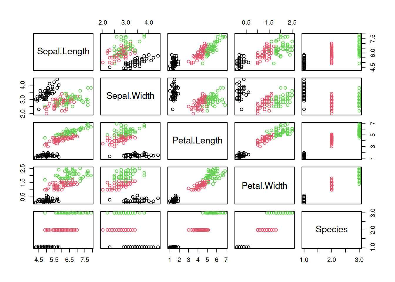
The Iris data is very clean, so we make the data a little messy by adding a random error to each variable and introduce a useless, completely random feature.
x[,1] <- x[,1] + rnorm(nrow(x))
x[,2] <- x[,2] + rnorm(nrow(x))
x[,3] <- x[,3] + rnorm(nrow(x))
x <- cbind(x[,-5],
           useless = mean(x[,1]) + rnorm(nrow(x)),
           Species = x[,5])

plot(x, col=x$Species)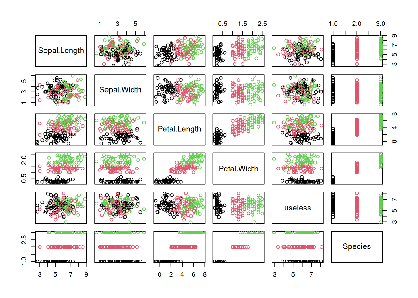
summary(x)
##   Sepal.Length   Sepal.Width     Petal.Length
##  Min.   :2.68   Min.   :0.611   Min.   :-0.713
##  1st Qu.:5.05   1st Qu.:2.306   1st Qu.: 1.876
##  Median :5.92   Median :3.171   Median : 4.102
##  Mean   :5.85   Mean   :3.128   Mean   : 3.781
##  3rd Qu.:6.70   3rd Qu.:3.945   3rd Qu.: 5.546
##  Max.   :8.81   Max.   :5.975   Max.   : 7.708
##   Petal.Width     useless           Species
##  Min.   :0.1   Min.   :2.92   setosa    :50
##  1st Qu.:0.3   1st Qu.:5.23   versicolor:50
##  Median :1.3   Median :5.91   virginica :50
##  Mean   :1.2   Mean   :5.88
##  3rd Qu.:1.8   3rd Qu.:6.56
##  Max.   :2.5   Max.   :8.11
head(x)
##     Sepal.Length Sepal.Width Petal.Length Petal.Width
## 85         2.980       1.464        5.227         1.5
## 104        5.096       3.044        5.187         1.8
## 30         4.361       2.832        1.861         0.2
## 53         8.125       2.406        5.526         1.5
## 143        6.372       1.565        6.147         1.9
## 142        6.526       3.697        5.708         2.3
##     useless    Species
## 85    5.712 versicolor
## 104   6.569  virginica
## 30    4.299     setosa
## 53    6.124 versicolor
## 143   6.553  virginica
## 142   5.222  virginica
We split the data into training and test data. Since the data is shuffled, we effectively perform holdout sampling. This is often not done in statistical applications, but we use the machine learning approach here.
train <- x[1:100,]
test <- x[101:150,]
Linear regression is done in R using the lm() (linear model) function which is
part of the R core package stats.
Like other modeling functions in R, lm() uses a formula interface. Here we create a formula
to predict Petal.Width by all other variables other than Species.
model1 <- lm(Petal.Width ~ Sepal.Length
            + Sepal.Width + Petal.Length + useless,
            data = train)
model1
##
## Call:
## lm(formula = Petal.Width ~ Sepal.Length + Sepal.Width + Petal.Length +
##     useless, data = train)
##
## Coefficients:
##  (Intercept)  Sepal.Length   Sepal.Width  Petal.Length
##     -0.20589       0.01957       0.03406       0.30814
##      useless
##      0.00392
The result is a model with the fitted \(\beta\) coefficients. More information can be displayed using the summary function.
summary(model1)
##
## Call:
## lm(formula = Petal.Width ~ Sepal.Length + Sepal.Width + Petal.Length +
##     useless, data = train)
##
## Residuals:
##     Min      1Q  Median      3Q     Max
## -1.0495 -0.2033  0.0074  0.2038  0.8564
##
## Coefficients:
##              Estimate Std. Error t value Pr(>|t|)
## (Intercept)  -0.20589    0.28723   -0.72     0.48
## Sepal.Length  0.01957    0.03265    0.60     0.55
## Sepal.Width   0.03406    0.03549    0.96     0.34
## Petal.Length  0.30814    0.01819   16.94   <2e-16 ***
## useless       0.00392    0.03558    0.11     0.91
## ---
## Signif. codes:
## 0 '***' 0.001 '**' 0.01 '*' 0.05 '.' 0.1 ' ' 1
##
## Residual standard error: 0.366 on 95 degrees of freedom
## Multiple R-squared:  0.778,  Adjusted R-squared:  0.769
## F-statistic: 83.4 on 4 and 95 DF,  p-value: <2e-16
The summary reports coefficient estimates and tests of whether each coefficient
is zero, conditional on the other predictors and the model assumptions. Here,
Petal.Length has a small p-value and the coefficient for useless is close
to zero. Such tests do not establish that a predictor is causally important,
and p-values can be optimistic after model selection.
R-squared (the coefficient of determination) is the proportion of the response variation explained by the fitted model on these data. Adjusted R-squared accounts for the number of predictors, but neither statistic is a substitute for evaluating predictions on held-out data. There is no universal cutoff for what counts as a good R-squared.
Plotting the model produces diagnostic plots (see plot.lm()). For example,
to check that the error term has a mean of 0 and is homoscedastic,
the residual vs. predicted value scatter plot
should have a red line that stays close to 0 and
not look like a funnel where they are increasing when the fitted values increase.
To check if the residuals are approximately normally distributed,
the Q-Q plot should be close to the straight diagonal line.
plot(model1, which = 1:2)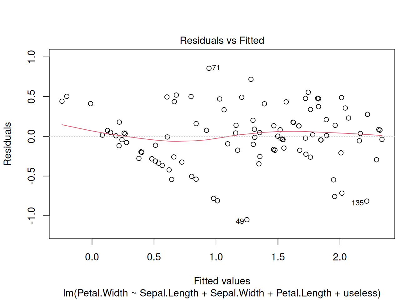
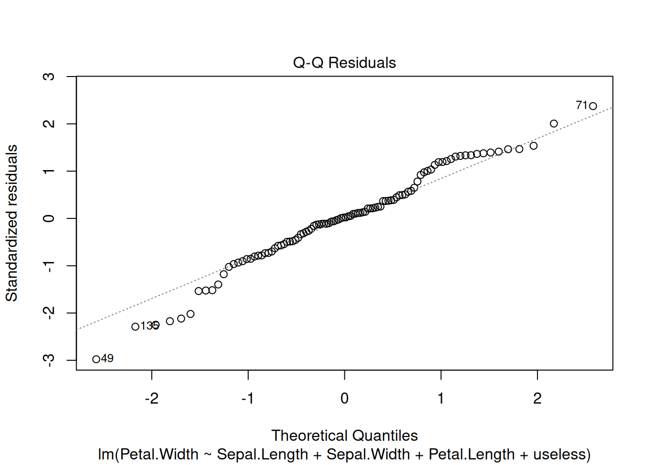
In this case, the two plots look fine.
B.5 Comparing Nested Models
Here we compare nested linear models. Models are nested when one model’s terms
are a subset of the other’s, with the same response and observations. We first
remove the random useless predictor.
model2 <- lm(Petal.Width ~ Sepal.Length +
               Sepal.Width + Petal.Length,
             data = train)
summary(model2)
##
## Call:
## lm(formula = Petal.Width ~ Sepal.Length + Sepal.Width + Petal.Length,
##     data = train)
##
## Residuals:
##     Min      1Q  Median      3Q     Max
## -1.0440 -0.2024  0.0099  0.1998  0.8513
##
## Coefficients:
##              Estimate Std. Error t value Pr(>|t|)
## (Intercept)   -0.1842     0.2076   -0.89     0.38
## Sepal.Length   0.0199     0.0323    0.62     0.54
## Sepal.Width    0.0339     0.0353    0.96     0.34
## Petal.Length   0.3080     0.0180   17.07   <2e-16 ***
## ---
## Signif. codes:
## 0 '***' 0.001 '**' 0.01 '*' 0.05 '.' 0.1 ' ' 1
##
## Residual standard error: 0.365 on 96 degrees of freedom
## Multiple R-squared:  0.778,  Adjusted R-squared:  0.771
## F-statistic:  112 on 3 and 96 DF,  p-value: <2e-16
The next example removes the intercept by adding -1 to the formula. This
changes the model assumptions and should only be done when a zero response at
zero predictors is scientifically appropriate.
model3 <- lm(Petal.Width ~ Sepal.Length +
               Sepal.Width + Petal.Length - 1,
             data = train)
summary(model3)
##
## Call:
## lm(formula = Petal.Width ~ Sepal.Length + Sepal.Width + Petal.Length -
##     1, data = train)
##
## Residuals:
##     Min      1Q  Median      3Q     Max
## -1.0310 -0.1961 -0.0051  0.2264  0.8246
##
## Coefficients:
##              Estimate Std. Error t value Pr(>|t|)
## Sepal.Length -0.00168    0.02122   -0.08     0.94
## Sepal.Width   0.01859    0.03073    0.61     0.55
## Petal.Length  0.30666    0.01796   17.07   <2e-16 ***
## ---
## Signif. codes:
## 0 '***' 0.001 '**' 0.01 '*' 0.05 '.' 0.1 ' ' 1
##
## Residual standard error: 0.364 on 97 degrees of freedom
## Multiple R-squared:  0.938,  Adjusted R-squared:  0.936
## F-statistic:  486 on 3 and 97 DF,  p-value: <2e-16
Here is a very simple model.
model4 <- lm(Petal.Width ~ Petal.Length -1,
             data = train)
summary(model4)
##
## Call:
## lm(formula = Petal.Width ~ Petal.Length - 1, data = train)
##
## Residuals:
##     Min      1Q  Median      3Q     Max
## -0.9774 -0.1957  0.0078  0.2536  0.8455
##
## Coefficients:
##              Estimate Std. Error t value Pr(>|t|)
## Petal.Length  0.31586    0.00822    38.4   <2e-16 ***
## ---
## Signif. codes:
## 0 '***' 0.001 '**' 0.01 '*' 0.05 '.' 0.1 ' ' 1
##
## Residual standard error: 0.362 on 99 degrees of freedom
## Multiple R-squared:  0.937,  Adjusted R-squared:  0.936
## F-statistic: 1.47e+03 on 1 and 99 DF,  p-value: <2e-16
For nested linear models, anova() performs a partial F-test of whether the
additional terms reduce residual error enough to support the larger model.
Compare only nested models fitted to the same observations. Here, models 1 and
2 form one nested pair, and models 3 and 4 form another. Models 2 and 3 differ
in their intercept structure and are not compared with the same test.
anova(model1, model2)
## Analysis of Variance Table
##
## Model 1: Petal.Width ~ Sepal.Length + Sepal.Width + Petal.Length + useless
## Model 2: Petal.Width ~ Sepal.Length + Sepal.Width + Petal.Length
##   Res.Df  RSS Df Sum of Sq    F Pr(>F)
## 1     95 12.8
## 2     96 12.8 -1  -0.00163 0.01   0.91
anova(model3, model4)
## Analysis of Variance Table
##
## Model 1: Petal.Width ~ Sepal.Length + Sepal.Width + Petal.Length - 1
## Model 2: Petal.Width ~ Petal.Length - 1
##   Res.Df  RSS Df Sum of Sq    F Pr(>F)
## 1     97 12.9
## 2     99 13.0 -2    -0.101 0.38   0.68
Interpret each test in light of its assumptions and the model purpose; a
non-significant result does not prove that the smaller model is correct. See
?anova.lm for details.
B.6 Stepwise Variable Selection
Stepwise variable selection performs backward (or forward) model selection for linear models and uses the smallest AIC (Akaike information criterion) to decide what variable to remove and when to stop.
s1 <- step(lm(Petal.Width ~ . -Species, data = train))
## Start:  AIC=-195.9
## Petal.Width ~ (Sepal.Length + Sepal.Width + Petal.Length + useless +
##     Species) - Species
##
##                Df Sum of Sq  RSS    AIC
## - useless       1       0.0 12.8 -197.9
## - Sepal.Length  1       0.0 12.8 -197.5
## - Sepal.Width   1       0.1 12.9 -196.9
## <none>                      12.8 -195.9
## - Petal.Length  1      38.6 51.3  -58.7
##
## Step:  AIC=-197.9
## Petal.Width ~ Sepal.Length + Sepal.Width + Petal.Length
##
##                Df Sum of Sq  RSS    AIC
## - Sepal.Length  1       0.1 12.8 -199.5
## - Sepal.Width   1       0.1 12.9 -198.9
## <none>                      12.8 -197.9
## - Petal.Length  1      38.7 51.5  -60.4
##
## Step:  AIC=-199.5
## Petal.Width ~ Sepal.Width + Petal.Length
##
##                Df Sum of Sq  RSS    AIC
## - Sepal.Width   1       0.1 12.9 -200.4
## <none>                      12.8 -199.5
## - Petal.Length  1      44.7 57.5  -51.3
##
## Step:  AIC=-200.4
## Petal.Width ~ Petal.Length
##
##                Df Sum of Sq  RSS    AIC
## <none>                      12.9 -200.4
## - Petal.Length  1      44.6 57.6  -53.2
summary(s1)
##
## Call:
## lm(formula = Petal.Width ~ Petal.Length, data = train)
##
## Residuals:
##     Min      1Q  Median      3Q     Max
## -0.9848 -0.1873  0.0048  0.2466  0.8343
##
## Coefficients:
##              Estimate Std. Error t value Pr(>|t|)
## (Intercept)    0.0280     0.0743    0.38     0.71
## Petal.Length   0.3103     0.0169   18.38   <2e-16 ***
## ---
## Signif. codes:
## 0 '***' 0.001 '**' 0.01 '*' 0.05 '.' 0.1 ' ' 1
##
## Residual standard error: 0.364 on 98 degrees of freedom
## Multiple R-squared:  0.775,  Adjusted R-squared:  0.773
## F-statistic:  338 on 1 and 98 DF,  p-value: <2e-16
Each table represents one step and shows the AIC when each variable is removed and
the one with the smallest AIC (in the first table useless) is removed. It stops
with a small model that only uses Petal.Length.
B.7 Modeling with Interaction Terms
Linear regression models the effect of each predictor separately
using a \(\beta\) coefficient.
What if two variables are only important together?
This is called an interaction between predictors and is modeled using
interaction terms.
In R’s formula() we can use : and *
to specify interactions. For linear regression, an interaction
means that a new predictor is created by multiplying the two original
predictors.
We can create a model with an interaction terms between Sepal.Length, Sepal.Width and
Petal.Length.
model5 <- lm(Petal.Width ~ Sepal.Length *
               Sepal.Width * Petal.Length,
             data = train)

summary(model5)
##
## Call:
## lm(formula = Petal.Width ~ Sepal.Length * Sepal.Width * Petal.Length,
##     data = train)
##
## Residuals:
##     Min      1Q  Median      3Q     Max
## -1.1064 -0.1882  0.0238  0.1767  0.8577
##
## Coefficients:
##                                       Estimate Std. Error
## (Intercept)                            -2.4207     1.3357
## Sepal.Length                            0.4484     0.2313
## Sepal.Width                             0.5983     0.3845
## Petal.Length                            0.7275     0.2863
## Sepal.Length:Sepal.Width               -0.1115     0.0670
## Sepal.Length:Petal.Length              -0.0833     0.0477
## Sepal.Width:Petal.Length               -0.0941     0.0850
## Sepal.Length:Sepal.Width:Petal.Length   0.0201     0.0141
##                                       t value Pr(>|t|)
## (Intercept)                             -1.81    0.073 .
## Sepal.Length                             1.94    0.056 .
## Sepal.Width                              1.56    0.123
## Petal.Length                             2.54    0.013 *
## Sepal.Length:Sepal.Width                -1.66    0.100 .
## Sepal.Length:Petal.Length               -1.75    0.084 .
## Sepal.Width:Petal.Length                -1.11    0.272
## Sepal.Length:Sepal.Width:Petal.Length    1.43    0.157
## ---
## Signif. codes:
## 0 '***' 0.001 '**' 0.01 '*' 0.05 '.' 0.1 ' ' 1
##
## Residual standard error: 0.36 on 92 degrees of freedom
## Multiple R-squared:  0.792,  Adjusted R-squared:  0.777
## F-statistic: 50.2 on 7 and 92 DF,  p-value: <2e-16
anova(model2, model5)
## Analysis of Variance Table
##
## Model 1: Petal.Width ~ Sepal.Length + Sepal.Width + Petal.Length
## Model 2: Petal.Width ~ Sepal.Length * Sepal.Width * Petal.Length
##   Res.Df  RSS Df Sum of Sq    F Pr(>F)
## 1     96 12.8
## 2     92 11.9  4     0.807 1.55   0.19
The models are nested, so the ANOVA comparison assesses whether the interaction terms improve fit over the main-effects model. Check predictive performance on held-out data before choosing a model for prediction.
B.8 Prediction
We make predictions for the held-out test set.
test[1:5,]
##     Sepal.Length Sepal.Width Petal.Length Petal.Width
## 128        8.017       1.541        3.515         1.8
## 92         5.268       4.064        6.064         1.4
## 50         5.461       4.161        1.117         0.2
## 134        6.055       2.951        4.599         1.5
## 8          4.900       5.096        1.086         0.2
##     useless    Species
## 128   6.110  virginica
## 92    4.938 versicolor
## 50    6.373     setosa
## 134   5.595  virginica
## 8     7.270     setosa
test[1:5,]$Petal.Width
## [1] 1.8 1.4 0.2 1.5 0.2
predict(model4, test[1:5,])
##    128     92     50    134      8
## 1.1104 1.9155 0.3529 1.4526 0.3429
The most used error measure for regression is the RMSE root-mean-square error.
RMSE <- function(predicted, true) mean((predicted-true)^2)^.5

RMSE(predict(model4, test), test$Petal.Width)
## [1] 0.3874
We can also visualize the quality of the prediction using a simple scatter plot of predicted vs. actual values.
plot(test[,"Petal.Width"], predict(model4, test),
  xlim=c(0,3), ylim=c(0,3),
  xlab = "actual", ylab = "predicted",
  main = "Petal.Width")
abline(0,1, col="red")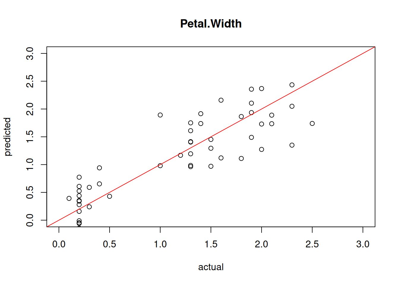
Perfect predictions would be on the red line, the farther they are away, the larger the error.
B.9 Using Nominal Variables
Dummy variables also called one-hot encoding in machine learning is used for factors (i.e., levels are translated into individual 0-1 variable). The first level of factors is automatically used as the reference and the other levels are presented as 0-1 dummy variables called contrasts.
levels(train$Species)
## [1] "setosa"     "versicolor" "virginica"
model.matrix() is used internally to create dummy variables when the design matrix
for the regression is created..
head(model.matrix(Petal.Width ~ ., data=train))
##     (Intercept) Sepal.Length Sepal.Width Petal.Length
## 85            1        2.980       1.464        5.227
## 104           1        5.096       3.044        5.187
## 30            1        4.361       2.832        1.861
## 53            1        8.125       2.406        5.526
## 143           1        6.372       1.565        6.147
## 142           1        6.526       3.697        5.708
##     useless Speciesversicolor Speciesvirginica
## 85    5.712                 1                0
## 104   6.569                 0                1
## 30    4.299                 0                0
## 53    6.124                 1                0
## 143   6.553                 0                1
## 142   5.222                 0                1
Note that there is no dummy variable for species Setosa, because it is
used as the reference (when the other two dummy variables are 0).
It is often useful to set the reference level.
A simple way is to use the
function relevel() to change which factor is listed first.
Let us perform model selection using AIC on the training data and then evaluate the final model on the held out test set to estimate the generalization error.
model6 <- step(lm(Petal.Width ~ ., data=train))
## Start:  AIC=-308.4
## Petal.Width ~ Sepal.Length + Sepal.Width + Petal.Length + useless +
##     Species
##
##                Df Sum of Sq   RSS  AIC
## - Sepal.Length  1      0.01  3.99 -310
## - Sepal.Width   1      0.01  3.99 -310
## - useless       1      0.02  4.00 -310
## <none>                       3.98 -308
## - Petal.Length  1      0.47  4.45 -299
## - Species       2      8.78 12.76 -196
##
## Step:  AIC=-310.2
## Petal.Width ~ Sepal.Width + Petal.Length + useless + Species
##
##                Df Sum of Sq   RSS  AIC
## - Sepal.Width   1      0.01  4.00 -312
## - useless       1      0.02  4.00 -312
## <none>                       3.99 -310
## - Petal.Length  1      0.49  4.48 -300
## - Species       2      8.82 12.81 -198
##
## Step:  AIC=-311.9
## Petal.Width ~ Petal.Length + useless + Species
##
##                Df Sum of Sq   RSS  AIC
## - useless       1      0.02  4.02 -313
## <none>                       4.00 -312
## - Petal.Length  1      0.48  4.48 -302
## - Species       2      8.95 12.95 -198
##
## Step:  AIC=-313.4
## Petal.Width ~ Petal.Length + Species
##
##                Df Sum of Sq   RSS  AIC
## <none>                       4.02 -313
## - Petal.Length  1      0.50  4.52 -304
## - Species       2      8.93 12.95 -200
model6
##
## Call:
## lm(formula = Petal.Width ~ Petal.Length + Species, data = train)
##
## Coefficients:
##       (Intercept)       Petal.Length  Speciesversicolor
##            0.1597             0.0664             0.8938
##  Speciesvirginica
##            1.4903
summary(model6)
##
## Call:
## lm(formula = Petal.Width ~ Petal.Length + Species, data = train)
##
## Residuals:
##     Min      1Q  Median      3Q     Max
## -0.7208 -0.1437  0.0005  0.1254  0.5460
##
## Coefficients:
##                   Estimate Std. Error t value Pr(>|t|)
## (Intercept)         0.1597     0.0441    3.62  0.00047 ***
## Petal.Length        0.0664     0.0192    3.45  0.00084 ***
## Speciesversicolor   0.8938     0.0746   11.98  < 2e-16 ***
## Speciesvirginica    1.4903     0.1020   14.61  < 2e-16 ***
## ---
## Signif. codes:
## 0 '***' 0.001 '**' 0.01 '*' 0.05 '.' 0.1 ' ' 1
##
## Residual standard error: 0.205 on 96 degrees of freedom
## Multiple R-squared:  0.93,   Adjusted R-squared:  0.928
## F-statistic:  427 on 3 and 96 DF,  p-value: <2e-16
RMSE(predict(model6, test), test$Petal.Width)
## [1] 0.1885
plot(test[,"Petal.Width"], predict(model6, test),
  xlim=c(0,3), ylim=c(0,3),
  xlab = "actual", ylab = "predicted",
  main = "Petal.Width")
abline(0,1, col="red")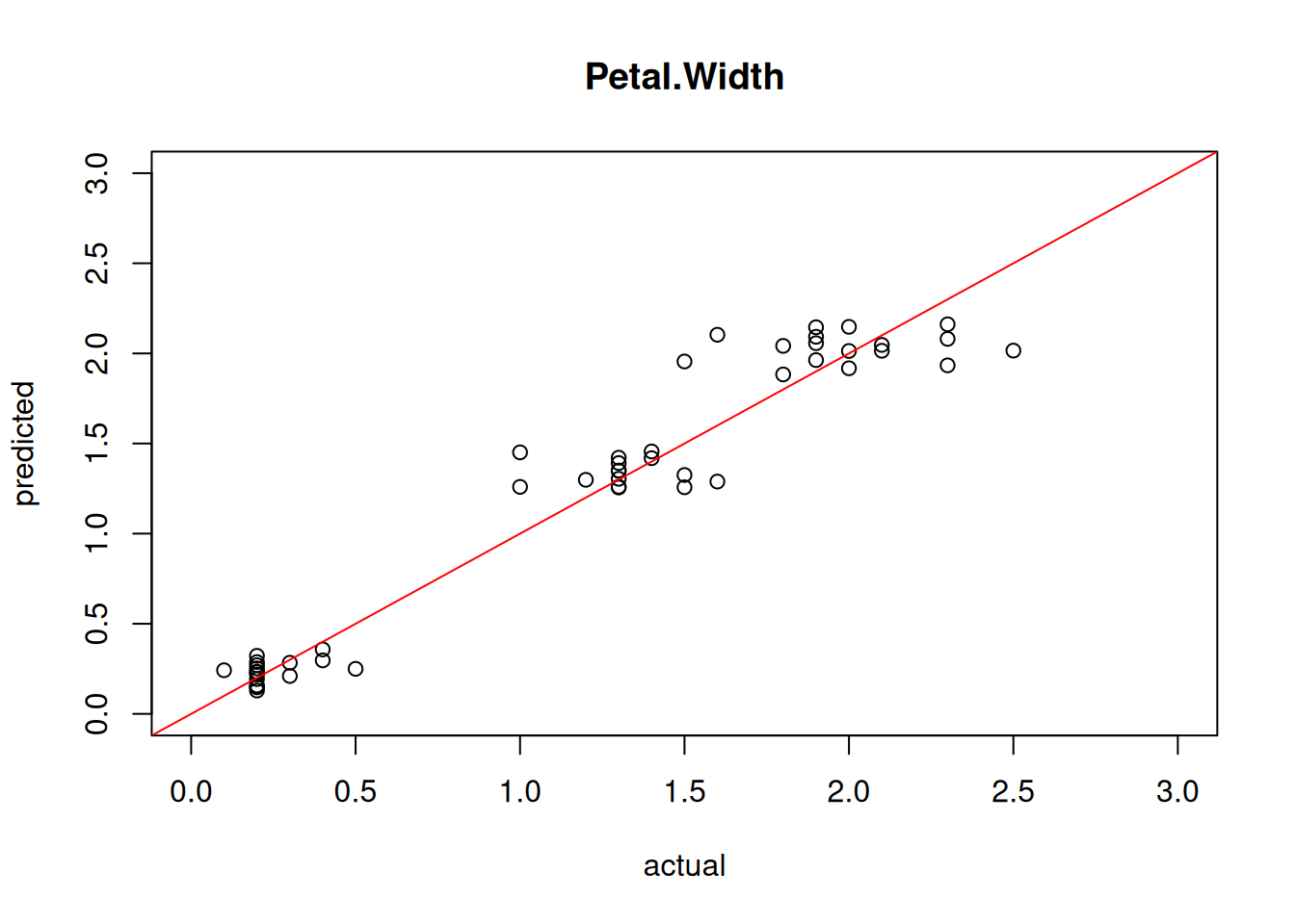
We see that the Species variable provides information to improve the regression model.
B.10 Alternative Regression Models
B.10.1 Regression Trees
Many models used for classification can also perform regression.
For example CART implemented in rpart performs regression
by estimating a value for each leaf note.
Regression is always performed by rpart() when the response variable
is not a factor().
library(rpart)
library(rpart.plot)
model7 <- rpart(Petal.Width ~ ., data = train,
control = rpart.control(cp = 0.01))
model7
## n= 100
##
## node), split, n, deviance, yval
## * denotes terminal node
##
## 1) root 100 57.5700 1.2190
## 2) Species=setosa 32 0.3797 0.2469 *
## 3) Species=versicolor,virginica 68 12.7200 1.6760
## 6) Species=versicolor 35 1.5350 1.3310 *
## 7) Species=virginica 33 2.6010 2.0420 *
rpart.plot(model7)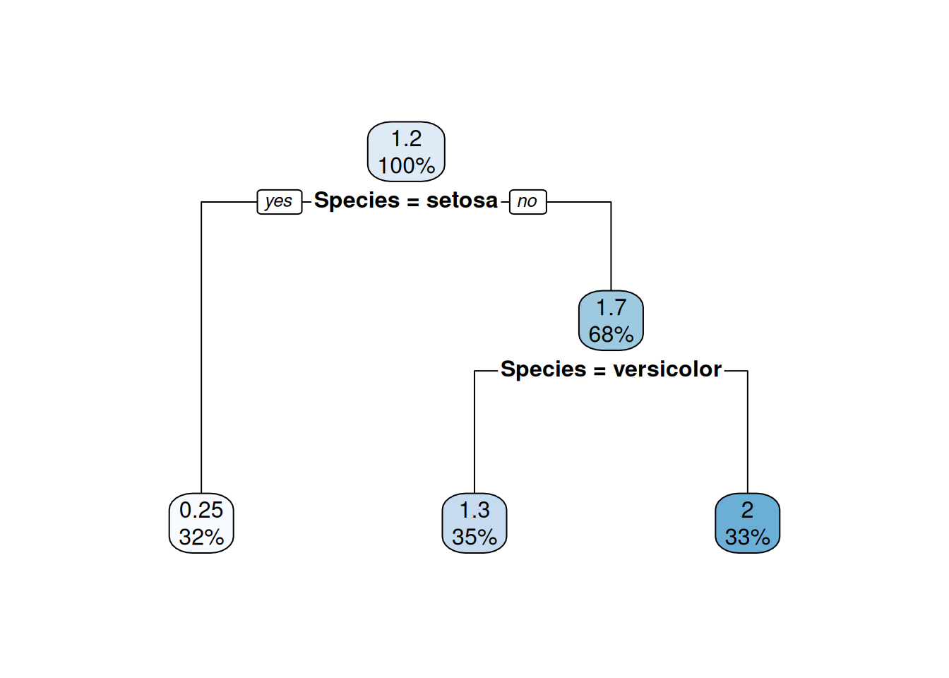 The regression tree shows the predicted value in as the top number in the node.
Also, remember that tree-based models automatically variable selection
by choosing the splits.
The regression tree shows the predicted value in as the top number in the node.
Also, remember that tree-based models automatically variable selection
by choosing the splits.Let’s evaluate the regression tree by calculating the RMSE.
And visualize the quality.
plot(test[,"Petal.Width"], pred,
  xlim = c(0,3), ylim = c(0,3),
  xlab = "actual", ylab = "predicted",
  main = "Petal.Width")
abline(0,1, col = "red")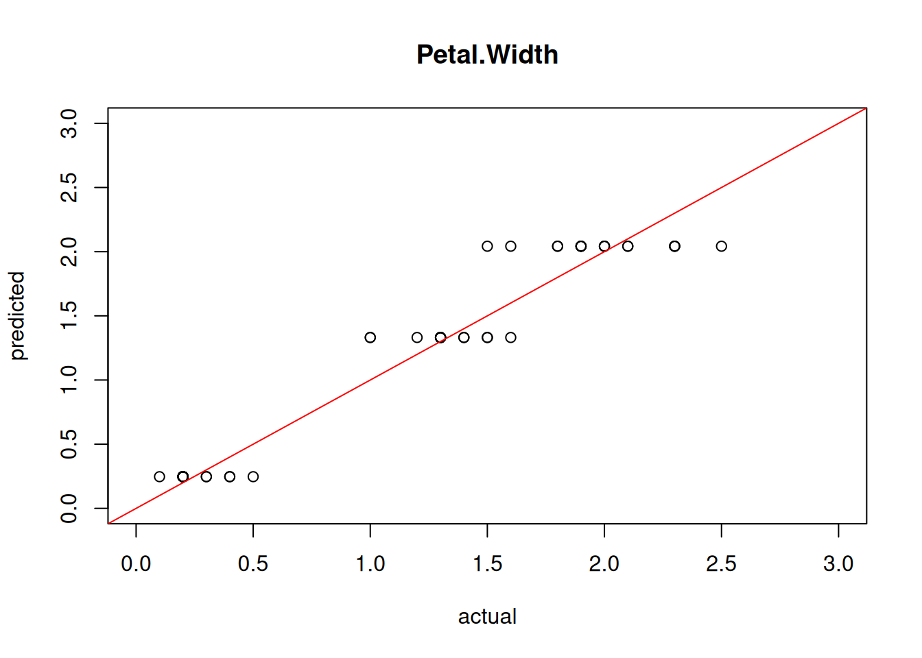
cor(test[,"Petal.Width"], pred)
## [1] 0.9717
The plot and the correlation coefficient indicate that the model is very good. In the plot we see an important property of this method which is that it predicts exactly the same value when the data falls in the same leaf node.
B.10.2 Regularized Regression
LASSO (least absolute shrinkage and selection operator)
uses L1 regularization to reduce to perform automatic variable selection.
The regularization adds a penalty for the L1 norm of the parameter vector \(\boldsymbol{\beta}\) (i.e., the summ of all
parameter values)
to the optimization. Increasing the weight of this penalty term (the weight is called \(\lambda\))
results in more and more weights being pushed to 0 which effectively reduces the number of
parameters used in the regression.
An implementation called
the elastic net
is available as the function lars() in package lars.
We create a design matrix (with dummy variables and interaction terms).
lm() did this automatically for us, but for this lars() implementation
we have to do it manually.
x <- model.matrix(~ . + Sepal.Length*Sepal.Width*Petal.Length ,
  data = train[, -4])
head(x)
##     (Intercept) Sepal.Length Sepal.Width Petal.Length
## 85            1        2.980       1.464        5.227
## 104           1        5.096       3.044        5.187
## 30            1        4.361       2.832        1.861
## 53            1        8.125       2.406        5.526
## 143           1        6.372       1.565        6.147
## 142           1        6.526       3.697        5.708
##     useless Speciesversicolor Speciesvirginica
## 85    5.712                 1                0
## 104   6.569                 0                1
## 30    4.299                 0                0
## 53    6.124                 1                0
## 143   6.553                 0                1
## 142   5.222                 0                1
##     Sepal.Length:Sepal.Width Sepal.Length:Petal.Length
## 85                     4.362                    15.578
## 104                   15.511                    26.431
## 30                    12.349                     8.114
## 53                    19.546                    44.900
## 143                    9.972                    39.168
## 142                   24.126                    37.253
##     Sepal.Width:Petal.Length
## 85                     7.650
## 104                   15.787
## 30                     5.269
## 53                    13.294
## 143                    9.620
## 142                   21.103
##     Sepal.Length:Sepal.Width:Petal.Length
## 85                                  22.80
## 104                                 80.45
## 30                                  22.98
## 53                                 108.01
## 143                                 61.30
## 142                                137.72
y <- train[, 4]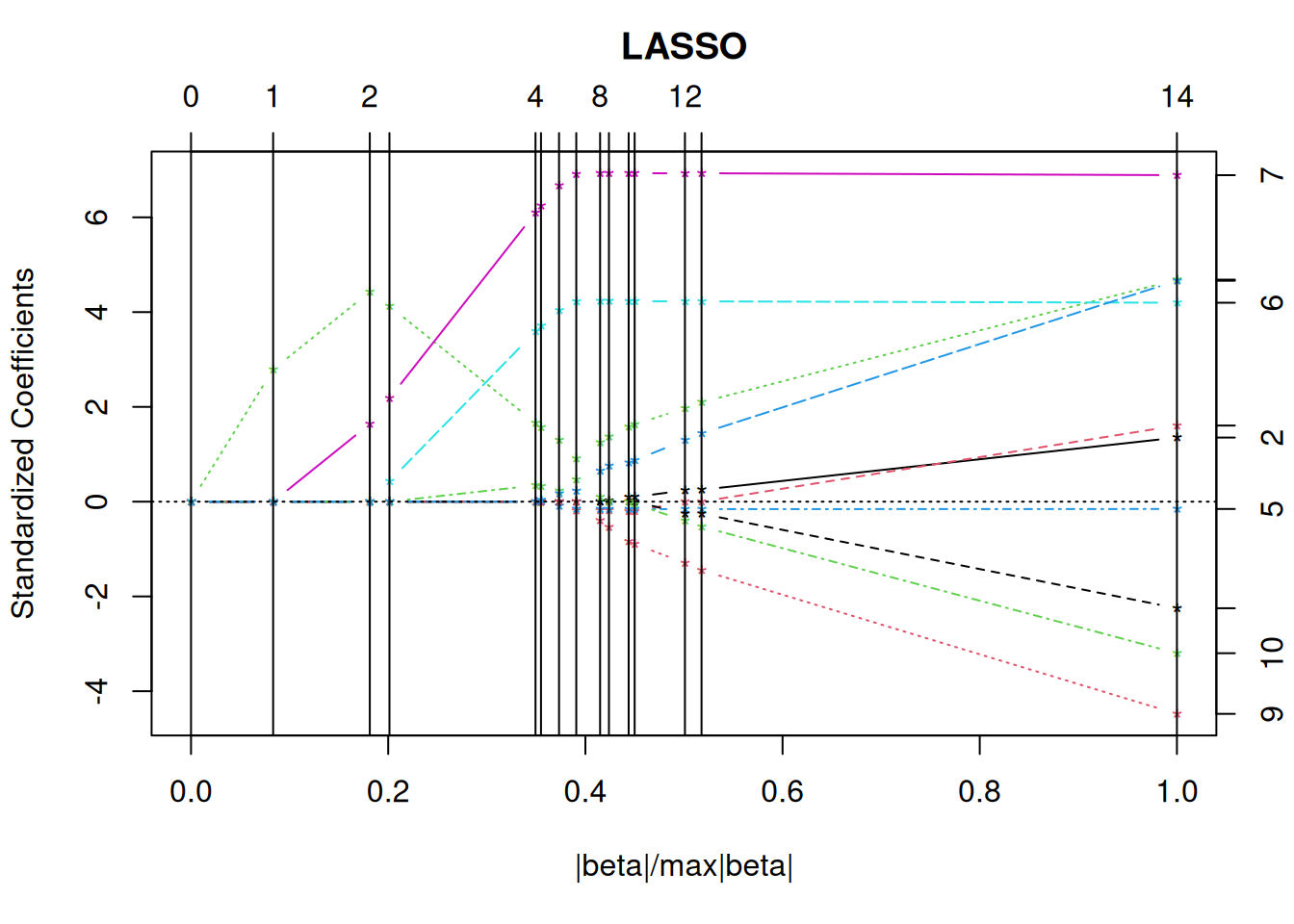
model_lars
##
## Call:
## lars(x = x, y = y)
## R-squared: 0.933
## Sequence of LASSO moves:
##      Petal.Length Speciesvirginica Speciesversicolor
## Var             4                7                 6
## Step            1                2                 3
##      Sepal.Width:Petal.Length
## Var                        10
## Step                        4
##      Sepal.Length:Sepal.Width:Petal.Length useless
## Var                                     11       5
## Step                                     5       6
##      Sepal.Width Sepal.Length:Petal.Length Sepal.Length
## Var            3                         9            2
## Step           7                         8            9
##      Sepal.Width:Petal.Length Sepal.Width:Petal.Length
## Var                       -10                       10
## Step                       10                       11
##      Sepal.Length:Sepal.Width Sepal.Width Sepal.Width
## Var                         8          -3           3
## Step                       12          13          14
The fitted model’s plot shows how variables are added (from left to right to the model).
The text output shoes that Petal.Length is the most important variable added to the model in step 1.
Then Speciesvirginica is added and so on.
This creates a sequence of nested models where one variable is added at a time.
To select the best model Mallows’s Cp statistic
can be used.
plot(model_lars, plottype = "Cp")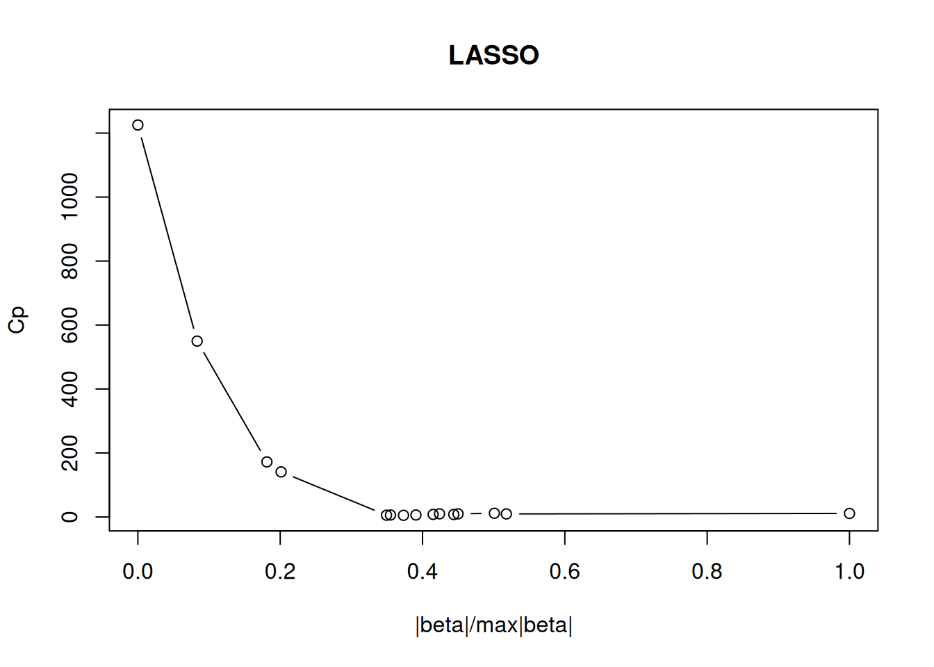
best <- which.min(model_lars$Cp)

coef(model_lars, s = best)
##                           (Intercept)
##                             0.0000000
##                          Sepal.Length
##                             0.0000000
##                           Sepal.Width
##                             0.0000000
##                          Petal.Length
##                             0.0603837
##                               useless
##                            -0.0086551
##                     Speciesversicolor
##                             0.8463786
##                      Speciesvirginica
##                             1.4181850
##              Sepal.Length:Sepal.Width
##                             0.0000000
##             Sepal.Length:Petal.Length
##                             0.0000000
##              Sepal.Width:Petal.Length
##                             0.0029688
## Sepal.Length:Sepal.Width:Petal.Length
##                             0.0003151
The variables that are not selected have a \(\beta\) coefficient of 0.
To make predictions with this model, we first have to convert the test data into a design matrix with the dummy variables and interaction terms.
x_test <- model.matrix(~ . + Sepal.Length*Sepal.Width*Petal.Length,
  data = test[, -4])
head(x_test)
##     (Intercept) Sepal.Length Sepal.Width Petal.Length
## 128           1        8.017       1.541        3.515
## 92            1        5.268       4.064        6.064
## 50            1        5.461       4.161        1.117
## 134           1        6.055       2.951        4.599
## 8             1        4.900       5.096        1.086
## 58            1        5.413       4.728        5.990
##     useless Speciesversicolor Speciesvirginica
## 128   6.110                 0                1
## 92    4.938                 1                0
## 50    6.373                 0                0
## 134   5.595                 0                1
## 8     7.270                 0                0
## 58    7.092                 1                0
##     Sepal.Length:Sepal.Width Sepal.Length:Petal.Length
## 128                    12.35                    28.182
## 92                     21.41                    31.944
## 50                     22.72                     6.102
## 134                    17.87                    27.847
## 8                      24.97                     5.319
## 58                     25.59                    32.424
##     Sepal.Width:Petal.Length
## 128                    5.417
## 92                    24.647
## 50                     4.649
## 134                   13.572
## 8                      5.531
## 58                    28.323
##     Sepal.Length:Sepal.Width:Petal.Length
## 128                                 43.43
## 92                                 129.83
## 50                                  25.39
## 134                                 82.19
## 8                                   27.10
## 58                                 153.31
Now we can compute the predictions.
predict(model_lars, x_test[1:5,], s = best)
## $s
## 6
## 7
##
## $fraction
##      6
## 0.4286
##
## $mode
## [1] "step"
##
## $fit
##    128     92     50    134      8
## 1.8237 1.5003 0.2505 1.9300 0.2439
The prediction is the fit element. We can calculate the RMSE.
And visualize the prediction.
plot(test[,"Petal.Width"],
     pred,
     xlim=c(0,3), ylim=c(0,3),
     xlab = "actual", ylab = "predicted",
     main = "Petal.Width")
abline(0,1, col = "red")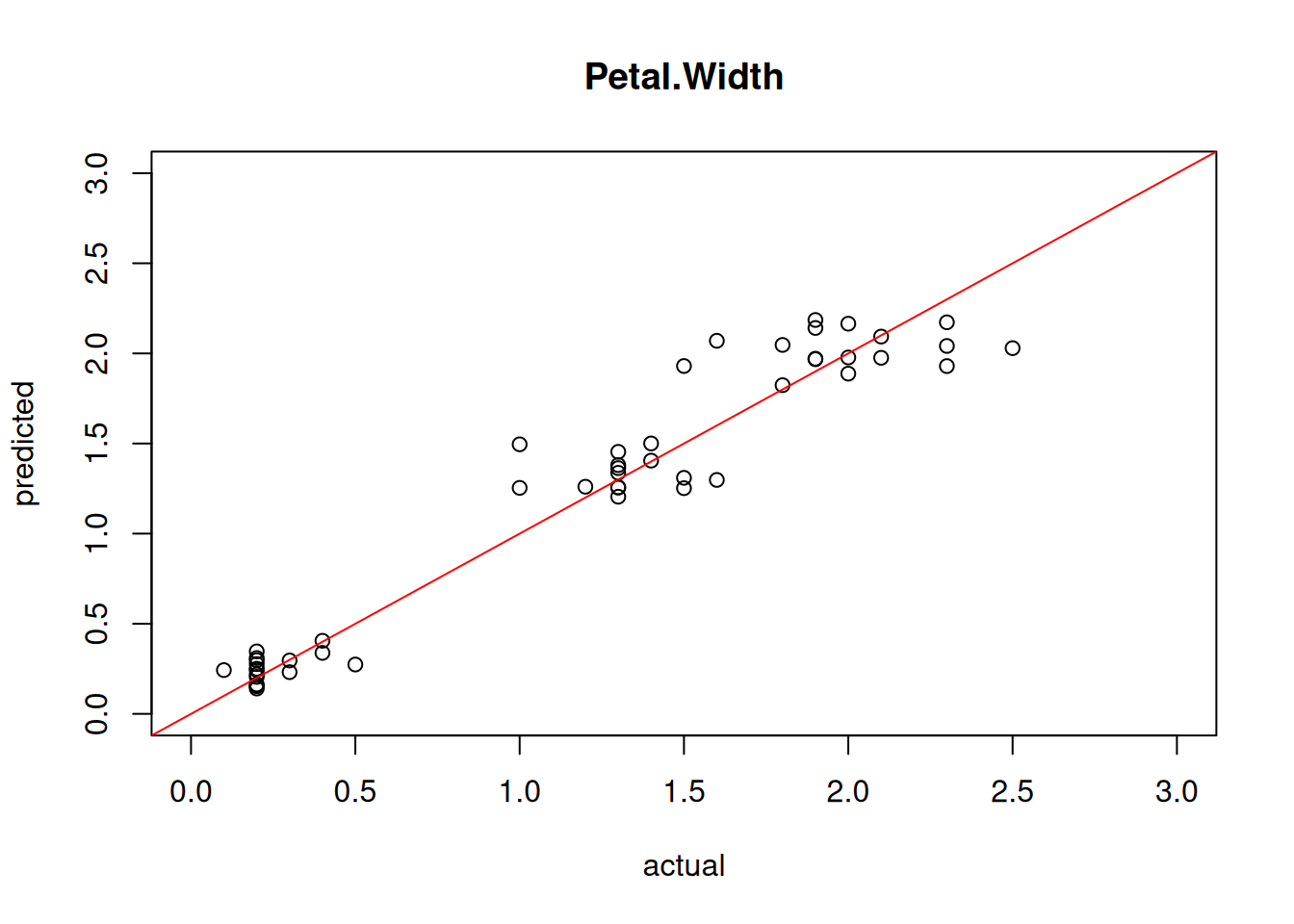
cor(test[,"Petal.Width"],
    pred)
## [1] 0.9686
The model shows good predictive power on the test set.
B.10.3 ANNs
Regression can be performed using artificial neural networks
with typically a linear final layer.
We will create a network using a single hidden layer
with 3 neurons (a manually tuned hyper parameter) and a linear output layer (set via linout).
library(nnet)

model_nnet <- nnet(Petal.Width ~ ., data = train, size = 3, linout = TRUE)
## # weights:  25
## initial  value 82.633473
## iter  10 value 14.094963
## iter  20 value 3.767394
## iter  30 value 3.372093
## iter  40 value 3.264074
## iter  50 value 3.224384
## iter  60 value 3.201191
## iter  70 value 3.182708
## iter  80 value 3.117583
## iter  90 value 3.087831
## iter 100 value 3.009898
## final  value 3.009898
## stopped after 100 iterations
model_nnet
## a 6-3-1 network with 25 weights
## inputs: Sepal.Length Sepal.Width Petal.Length useless Speciesversicolor Speciesvirginica
## output(s): Petal.Width
## options were - linear output unitsAnd visualize the quality.
plot(test[,"Petal.Width"], pred,
  xlim = c(0,3), ylim = c(0,3),
  xlab = "actual", ylab = "predicted",
  main = "Petal.Width")
abline(0,1, col = "red")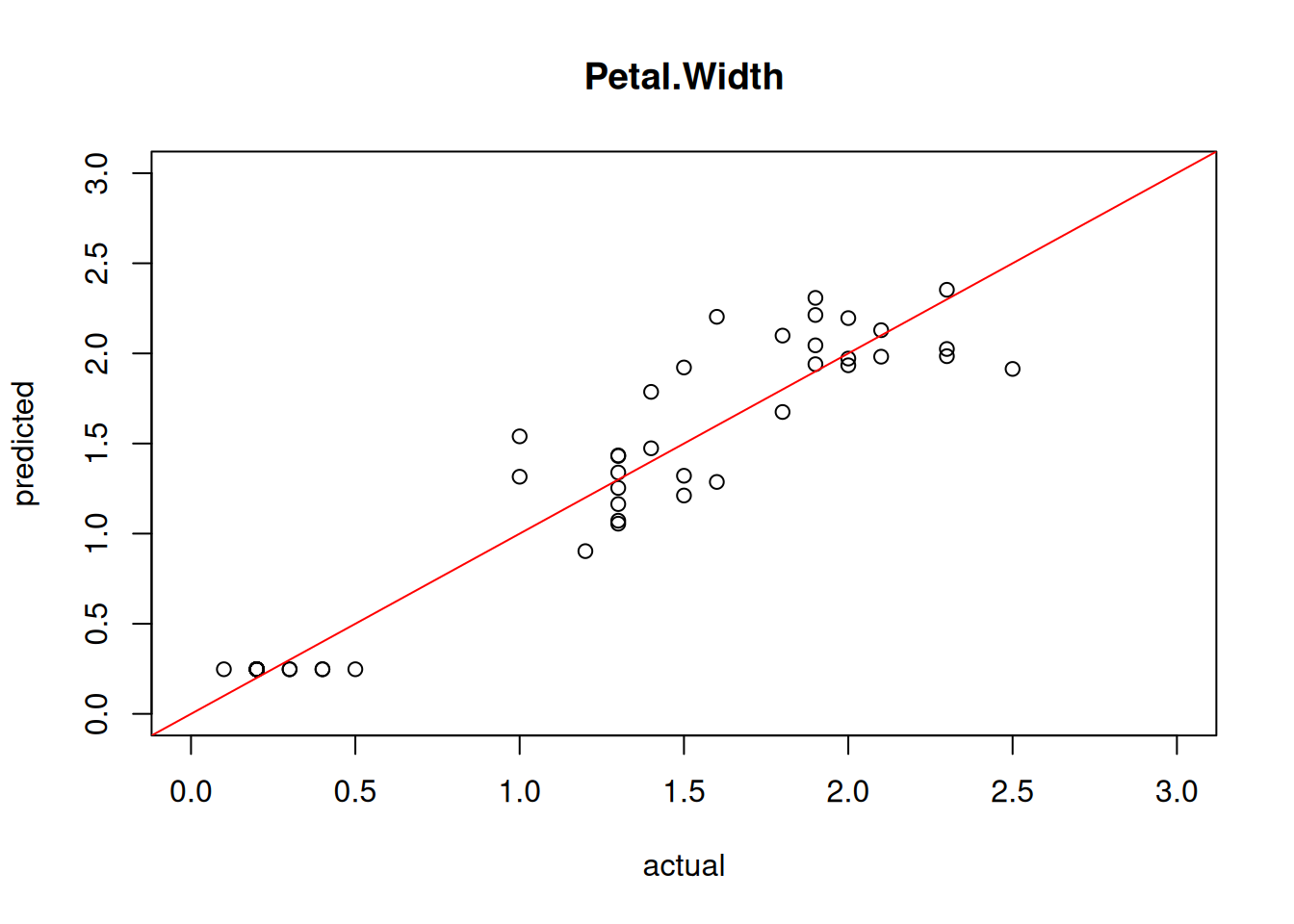
cor(test[,"Petal.Width"], pred)
##        [,1]
## [1,] 0.9546
Note: It is often necessary to scale the inputs to the ANN so it can learn effectively. It is very popular to scale all inputs to the ranges \([0,1]\) or \([-1,1]\). The ranges of the Iris dataset are fine, so there was no need for scaling.
B.11 Exercises
We will again use the Palmer penguin data for the exercises.
library(palmerpenguins)
##
## Attaching package: 'palmerpenguins'
## The following objects are masked from 'package:datasets':
##
##     penguins, penguins_raw
head(penguins)
## # A tibble: 6 × 8
##   species island    bill_length_mm bill_depth_mm
##   <fct>   <fct>              <dbl>         <dbl>
## 1 Adelie  Torgersen           39.1          18.7
## 2 Adelie  Torgersen           39.5          17.4
## 3 Adelie  Torgersen           40.3          18
## 4 Adelie  Torgersen           NA            NA
## 5 Adelie  Torgersen           36.7          19.3
## 6 Adelie  Torgersen           39.3          20.6
## # ℹ 4 more variables: flipper_length_mm <int>,
## #   body_mass_g <int>, sex <fct>, year <int>
Create an R markdown document that performs the following:
Create a linear regression model to predict the weight of a penguin (
body_mass_g).How high is the R-squared. What does it mean.
What variables are significant, what are not?
Use stepwise variable selection to remove unnecessary variables.
-
Predict the weight for the following new penguin:
library("tibble")

new_penguin <- tibble(
  species = factor("Adelie",
    levels = c("Adelie", "Chinstrap", "Gentoo")),
  island = factor("Dream",
    levels = c("Biscoe", "Dream", "Torgersen")),
 bill_length_mm = 39.8,
 bill_depth_mm = 19.1,
 flipper_length_mm = 184,
 body_mass_g = NA,
 sex = factor("male", levels = c("female", "male")),
 year = 2007
)
new_penguin
## # A tibble: 1 × 8
##   species island bill_length_mm bill_depth_mm
##   <fct>   <fct>           <dbl>         <dbl>
## 1 Adelie  Dream            39.8          19.1
## # ℹ 4 more variables: flipper_length_mm <dbl>,
## #   body_mass_g <lgl>, sex <fct>, year <dbl>
Create a regression tree. Look at the tree and explain what it does. Then use the regression tree to predict the weight for the above penguin.
A good answer should explain the response and predictors, interpret coefficients with their units and reference levels, and describe what R-squared and the significance results do and do not establish. Explain the stepwise selection process, report the prediction for the specified penguin, and describe the tree’s splits and prediction. Where possible, assess prediction quality on data not used to fit or select the model.
B.12 Chapter Summary
Regression predicts a numeric response from one or more explanatory variables. The chapter builds a linear model, interprets coefficients, compares nested models, and demonstrates stepwise variable selection and interaction terms. It shows how to generate predictions, work with nominal predictors, and assess models on data not used for fitting or selection. When ordinary linear regression is not suitable, regression trees, regularized regression, and artificial neural networks offer alternatives; other regression approaches are also surveyed. Model assumptions, complexity, and evaluation data should guide comparisons.
B.13 Key Terms
- Response: the numeric outcome a regression model predicts.
- Coefficient: the estimated change in response associated with a predictor, holding other model terms fixed.
- Interaction: a model term allowing the effect of one predictor to depend on another predictor.
- Residual: the difference between an observed response and its fitted value.
- Regularization: a method that constrains model coefficients to reduce overfitting.