Plot a 2-State or 3-State Projection of the Belief Space

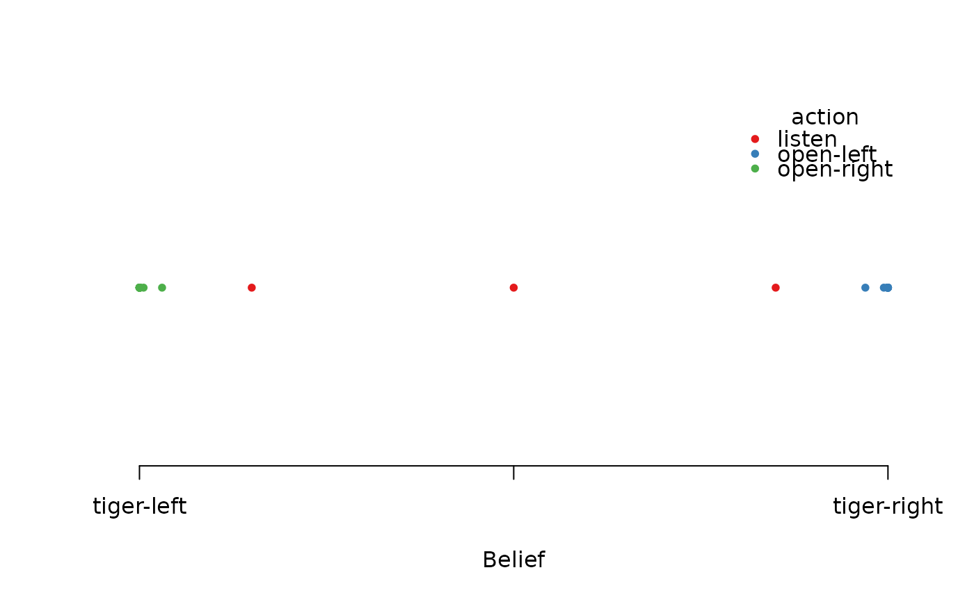
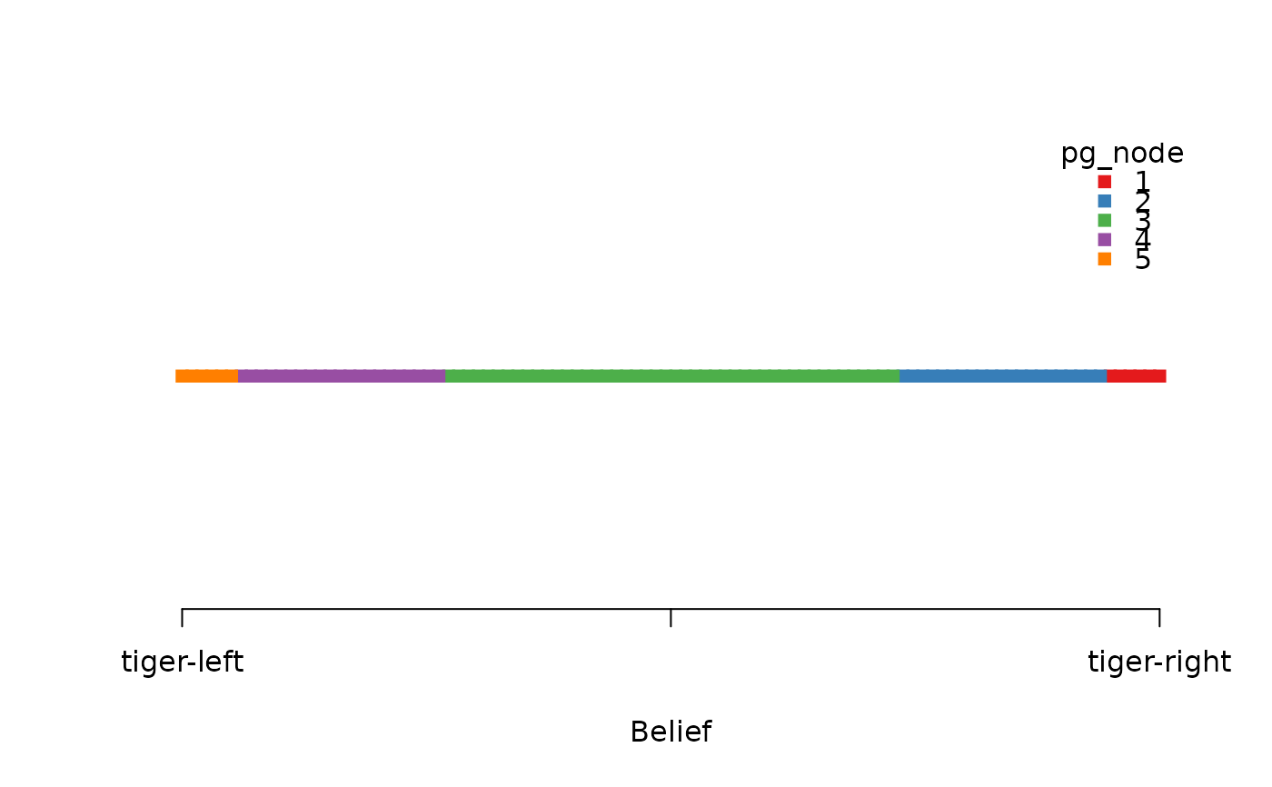
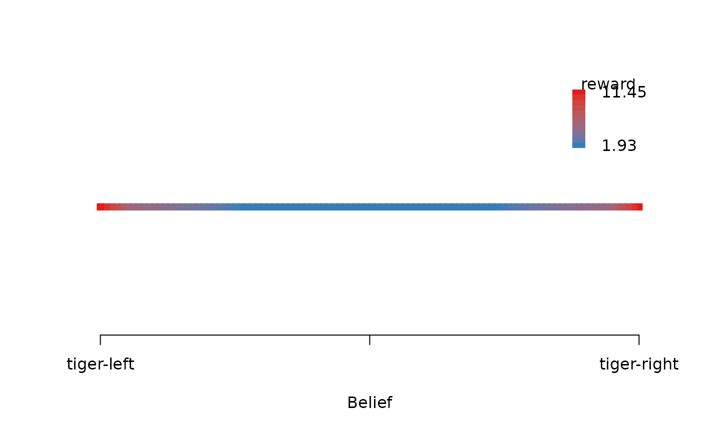
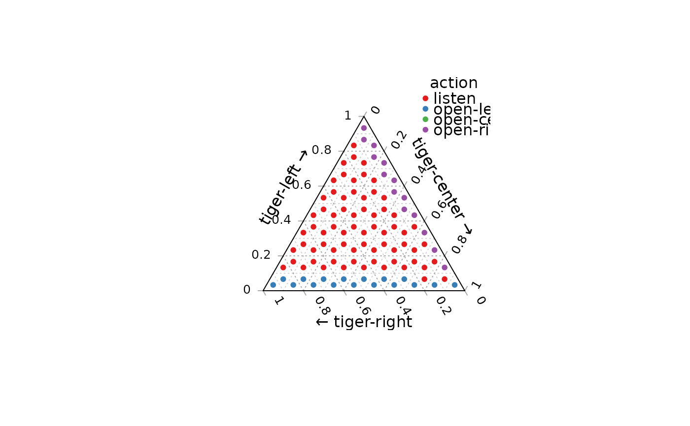
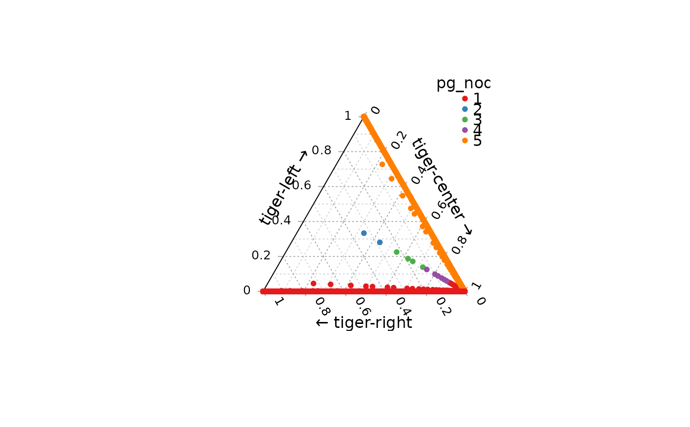
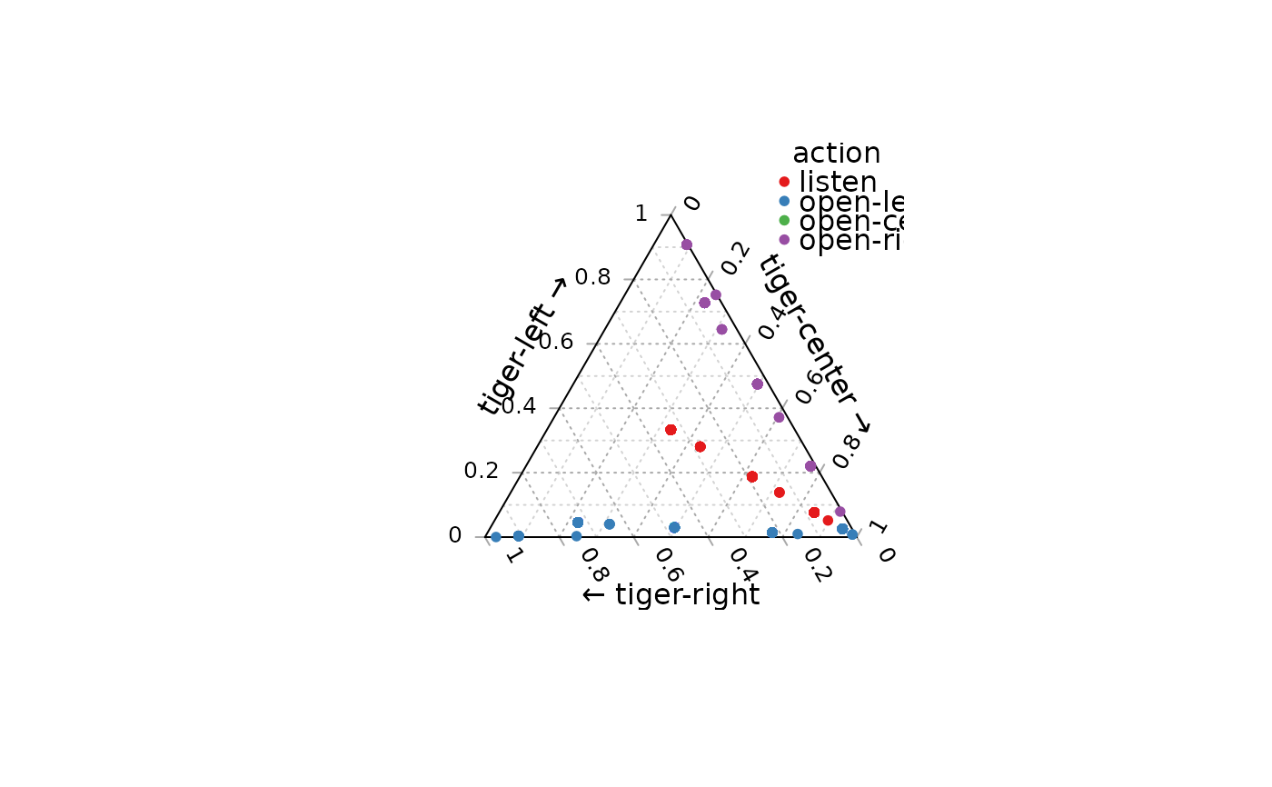
Plots the optimal action, the node in the policy graph or the reward for a given set of belief points on a line (2 states) or as a ternary plot (3 states). If no points are given, points are sampled using a regular arrangement or randomly from the (projected) belief space.

Usage

plot_belief_space(
  model,
  projection = NULL,
  epoch = 1,
  sample = "regular",
  n = 100,
  what = c("action", "pg_node", "reward"),
  legend = TRUE,
  pch = 20,
  col = NULL,
  jitter = 0,
  oneD = TRUE,
  ...
)

Arguments

model: a solved POMDP.
projection: Sample in a projected belief space. See projection() for details.
epoch: display this epoch.
sample: a matrix with belief points as rows or a character string specifying the method used for sample_belief_space().
n: number of points sampled.
what: what to plot.
legend: logical; add a legend? If the legend is covered by the plot then you need to increase the plotting region of the plotting device.
pch: plotting symbols.
col: plotting colors.
jitter: jitter amount for 2-state belief spaces (good values are between 0 and 1, while using ylim = c(0,1)).
oneD: plot projections on two states in one dimension.
...: additional arguments are passed on to plot for 2-state or TerneryPlot for 3-state plots.

Value

Returns invisibly the sampled points.

Author

Michael Hahsler

Examples

# two-state POMDP
data("Tiger")
sol <- solve_POMDP(Tiger)

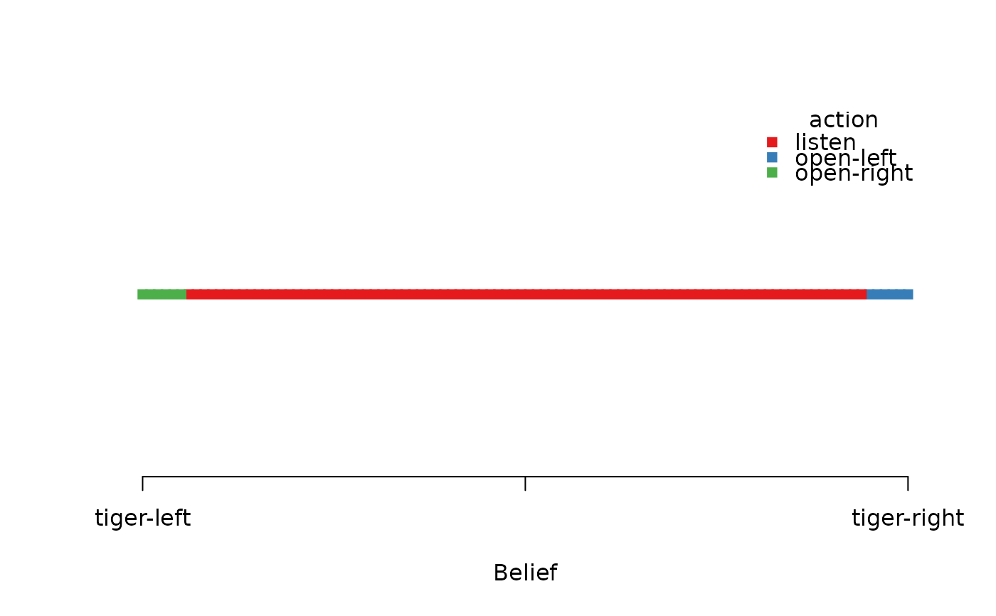
plot_belief_space(sol, pch = 15)

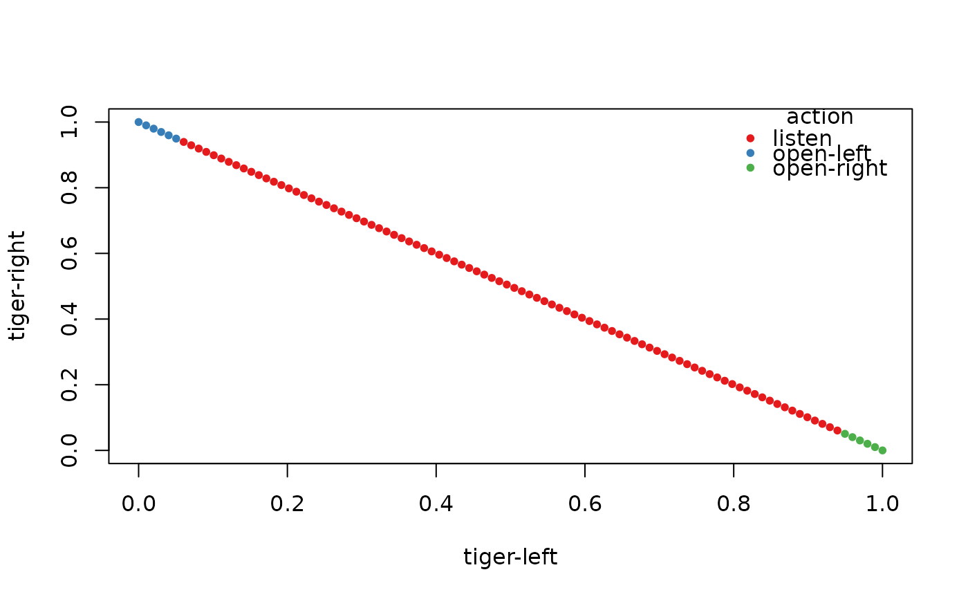
plot_belief_space(sol, oneD = FALSE)

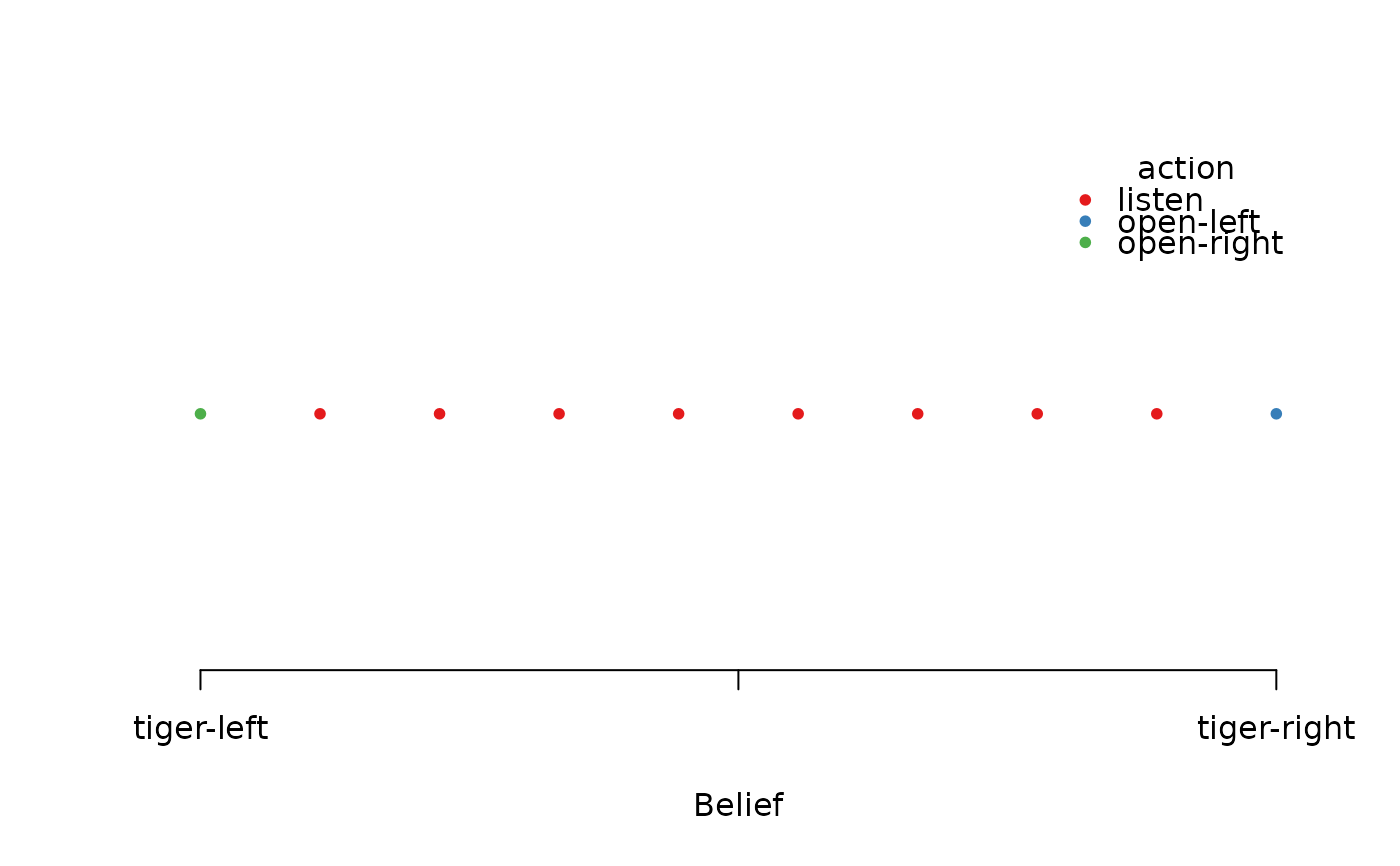
plot_belief_space(sol, n = 10)

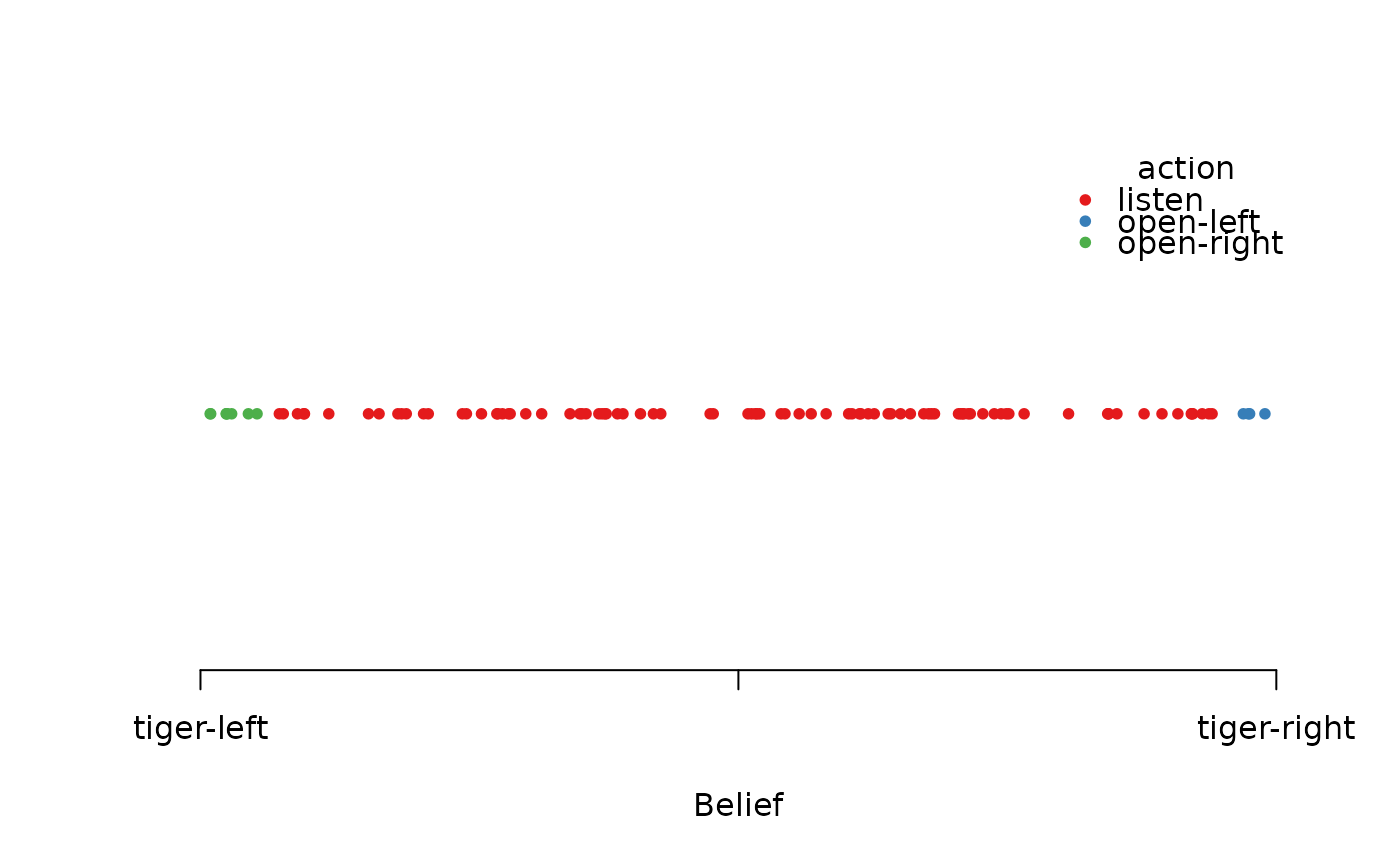
plot_belief_space(sol, n = 100, sample = "random")


# plot the belief points used by the grid-based solver
plot_belief_space(sol, sample = sol$solution$belief_points_solver)


# plot different measures
plot_belief_space(sol, what = "pg_node", pch = 15)

plot_belief_space(sol, what = "reward", pch = 15)


# three-state POMDP
# Note: If the plotting region is too small then the legend might run into the plot
data("Three_doors")
sol <- solve_POMDP(Three_doors)
sol
#> POMDP, list - 3-Door Tiger Problem
#>   Discount factor: 0.75
#>   Horizon: Inf epochs
#>   Size: 3 states / 4 actions / 3 obs.
#>   Start: uniform
#>   Solved:
#>     Method: ‘grid’
#>     Solution converged: TRUE
#>     # of alpha vectors: 5
#>     Total expected reward: 5.068327
#> 
#>   List components: ‘name’, ‘discount’, ‘horizon’, ‘states’, ‘actions’,
#>     ‘observations’, ‘transition_prob’, ‘observation_prob’, ‘reward’,
#>     ‘start’, ‘info’, ‘solution’

# plotting needs the suggested package Ternary for 3-state plots
if ("Ternary" %in% installed.packages()) {
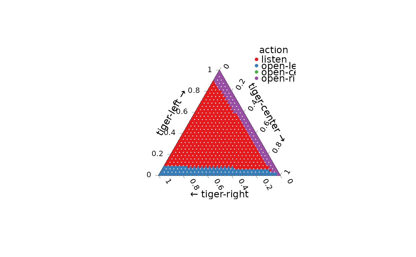
plot_belief_space(sol)
plot_belief_space(sol, n = 1024)
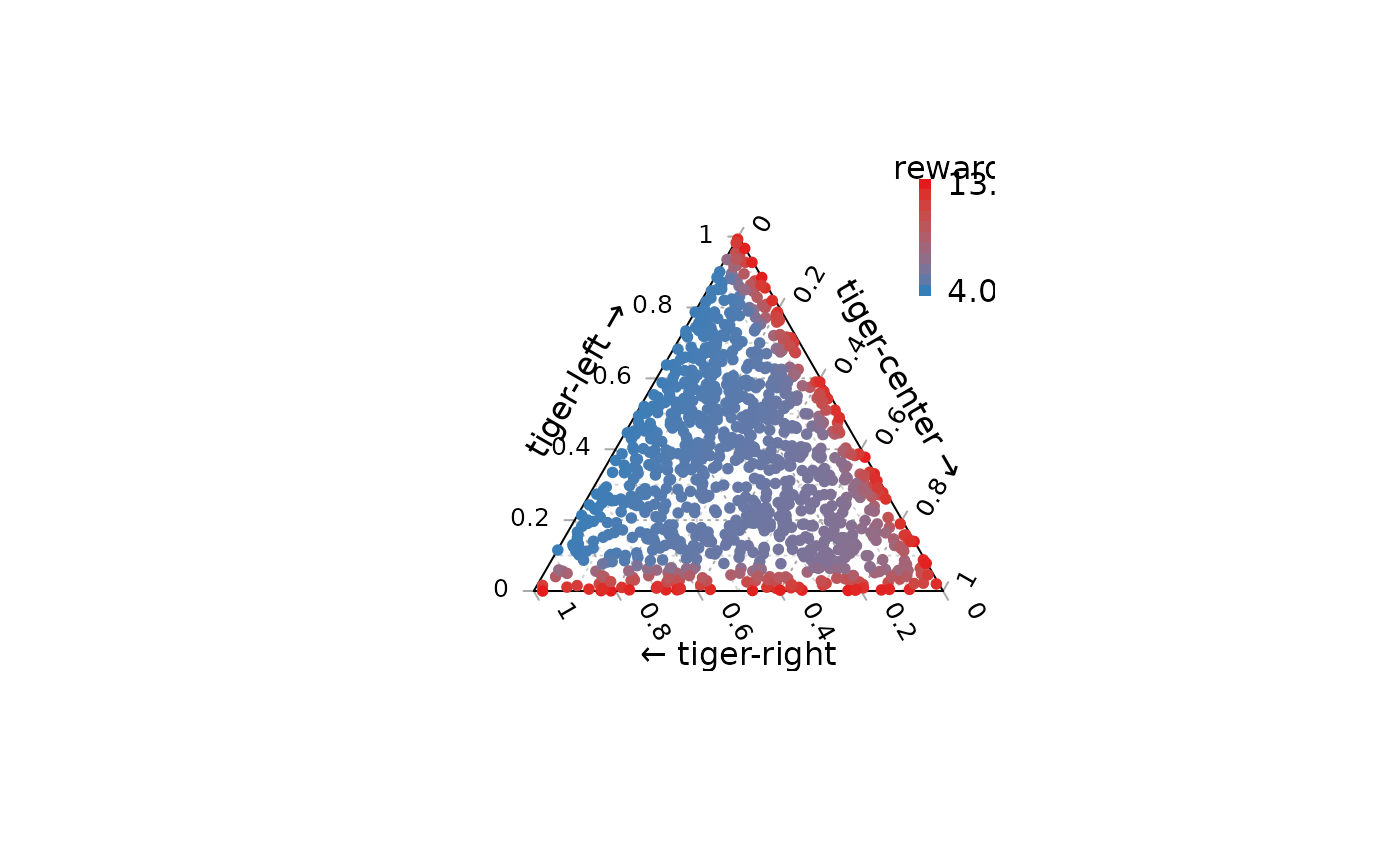
plot_belief_space(sol, what = "reward", sample = "random", n = 1000)

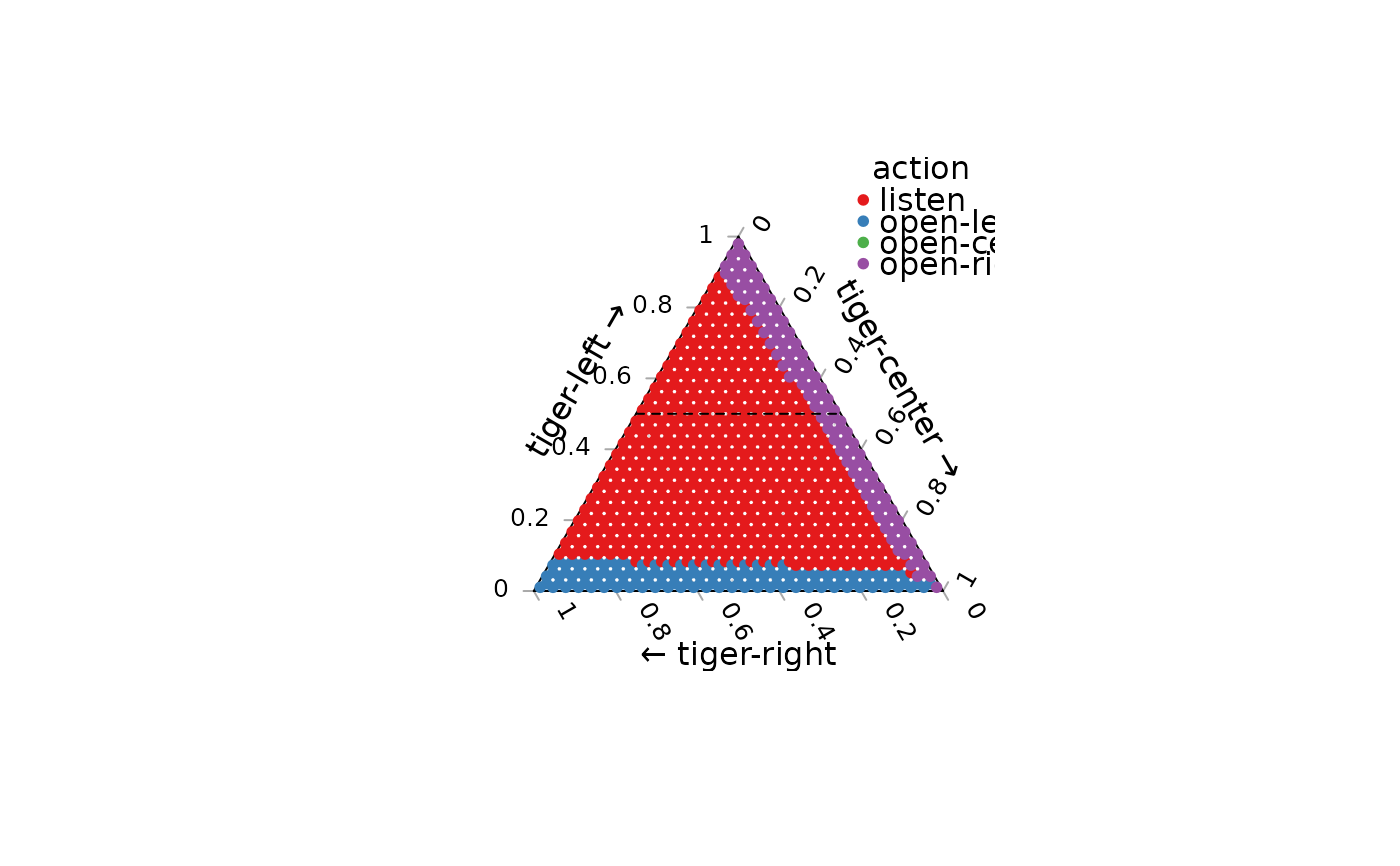
# holding tiger-left constant at .5 follows this line in the ternary plot 
plot_belief_space(sol, n = 1024)
Ternary::TernaryLines(list(c(.5, 0, .5), c(.5, .5, 0)), col = "black", lty = 2)

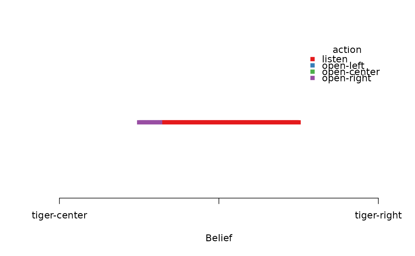
# we can plot the projection for this line 
plot_belief_space(sol, what = "action", n = 100, pch = 15, 
  projection = c("tiger-left" = .5))

# plot the belief points used by the grid-based solver
plot_belief_space(sol, sample = sol$solution$belief_points_solver, what = "pg_node")

# plot the belief points obtained using simulated trajectories with an epsilon-greedy policy.
# Note that we only use n = 50 to save time.
plot_belief_space(sol, 
  sample = simulate_POMDP(sol, n = 50, horizon = 100,
    epsilon = 0.1, return_beliefs = TRUE)$belief_states)
}








# plot a 3-state belief space using ggtern (ggplot2)
if (FALSE) { # \dontrun{
library(ggtern)
samp <- sample_belief_space(sol, n = 1000)
df <- cbind(as.data.frame(samp), reward_node_action(sol, belief = samp))
df$pg_node <- factor(df$pg_node)

ggtern(df, aes(x = `tiger-left`, y = `tiger-center`, z = `tiger-right`)) +
  geom_point(aes(color = pg_node), size = 2)

ggtern(df, aes(x = `tiger-left`, y = `tiger-center`, z = `tiger-right`)) +
  geom_point(aes(color = action), size = 2)

ggtern(df, aes(x = `tiger-left`, y = `tiger-center`, z = `tiger-right`)) +
  geom_point(aes(color = reward), size = 2)
} # }