Hodson's Munsingen Data Set

This data set contains a grave times artifact incidence matrix for the Celtic Münsingen-Rain cemetery in Switzerland as provided by Hodson (1968) and published by Kendall 1971.

Format

A 59 x 70 0-1 matrix. Rows (graves) and columns (artifacts) are in the order determined by Hodson (1968).

References

Hodson, F.R. (1968). The La Tene Cemetery at Münsingen-Rain, Stämpfli, Bern.

Kendall, D.G. (1971): Seriation from abundance matrices. In: Hodson, F.R., Kendall, D.G. and Tautu, P., (Editors), Mathematics in the Archaeological and Historical Sciences, Edinburgh University Press, Edinburgh, 215–232.

Examples

data("Munsingen")

## Seriation method after Kendall (1971)
## Kendall's square symmetric matrix S and SoS
S <- function(x, w = 1) {
  sij <- function(i , j) w * sum(pmin(x[i,], x[j,]))
  h <- nrow(x)
  r <- matrix(ncol = h, nrow =h)
  for(i in 1:h) for (j in 1:h)  r[i,j] <- sij(i,j)
  r
}

SoS <- function(x) S(S(x))

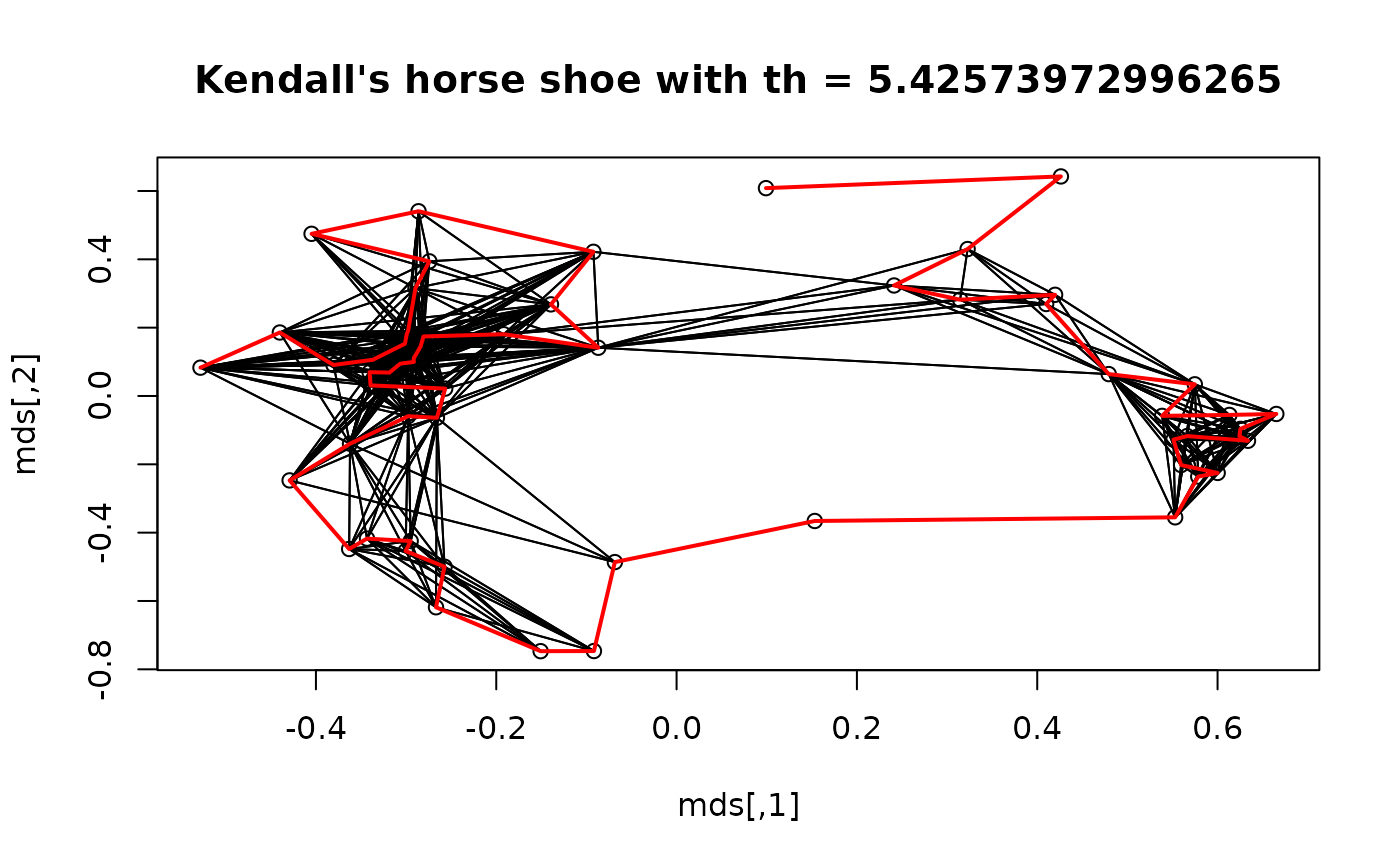
## Kendall's horse shoe (Hamiltonian arc)
horse_shoe_plot <- function(mds, sigma, threshold = mean(sigma), ...) {
    plot(mds, main = paste("Kendall's horse shoe with th =", threshold), ...)
    l <- which(sigma > threshold, arr.ind=TRUE)
    for(i in 1:nrow(l))  lines(rbind(mds[l[i,1],], mds[l[i,2],]))
}

## shuffle data
x <- Munsingen[sample(nrow(Munsingen)),]

## calculate matrix and do isoMDS (from package MASS)
sigma <- SoS(x)
library("MASS")
mds <- isoMDS(1/(1+sigma))$points
#> initial  value 21.862779 
#> iter   5 value 15.918885
#> iter  10 value 15.609393
#> iter  10 value 15.600691
#> iter  10 value 15.597381
#> final  value 15.597381 
#> converged

## plot Kendall's horse shoe
horse_shoe_plot(mds, sigma)

## find order using a TSP
library("TSP")
tour <- solve_TSP(insert_dummy(TSP(dist(mds)), label = "cut"),
    method = "2-opt", control = list(rep = 15))
#> Warning: executing %dopar% sequentially: no parallel backend registered
tour <- cut_tour(tour, "cut")
lines(mds[tour,], col = "red", lwd = 2)


## create and plot order
order <- ser_permutation(tour, 1:ncol(x))
bertinplot(x, order, options= list(panel=panel.circles,
    rev = TRUE))
#> Warning: eval(expr, envir): Unknown control parameter(s) ‘options’ are ignored. Rerun with verbose = TRUE.


## compare criterion values
rbind(
    random = criterion(x),
    reordered = criterion(x, order),
    Hodson = criterion(Munsingen)
   )
#>                 Cor_R  ME Moore_stress Neumann_stress
#> random    -0.01319356 143         3484           1556
#> reordered -0.44671351 226         2738           1258
#> Hodson     0.94236369 239         2574           1206

Format

References

See also

Examples