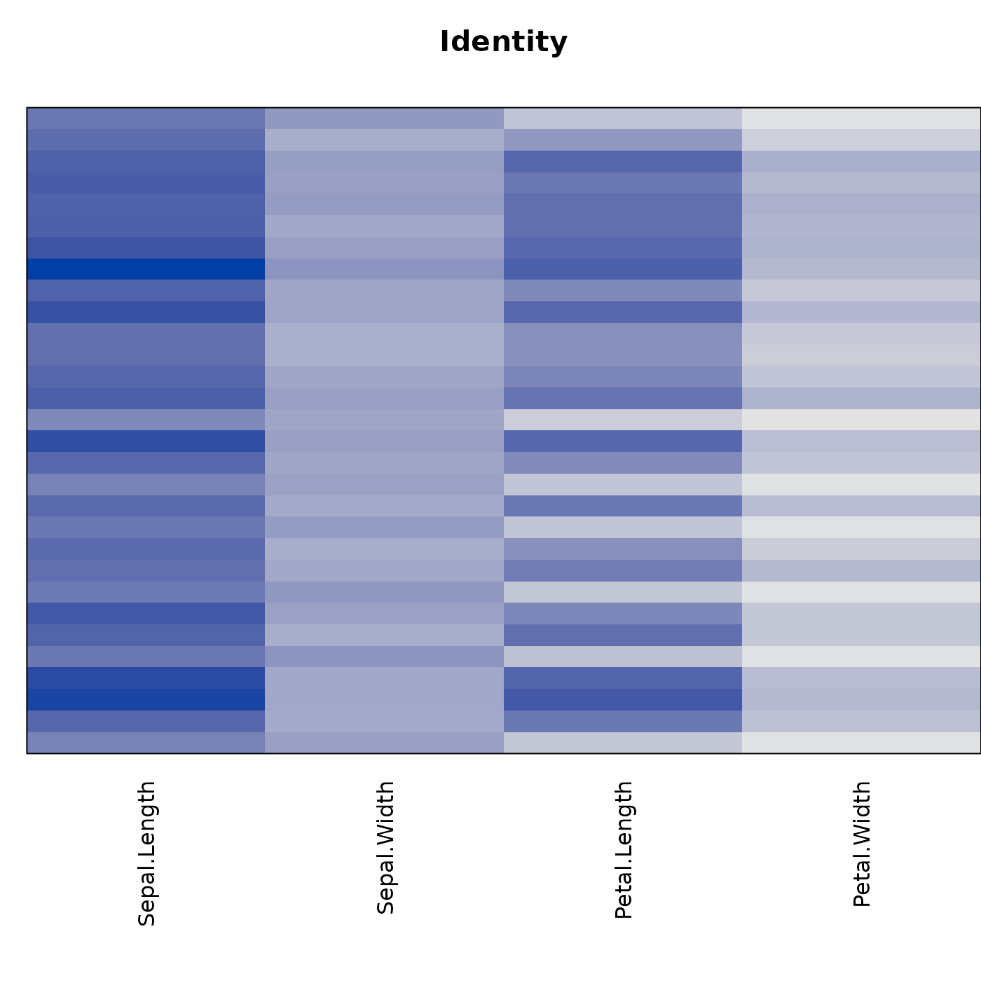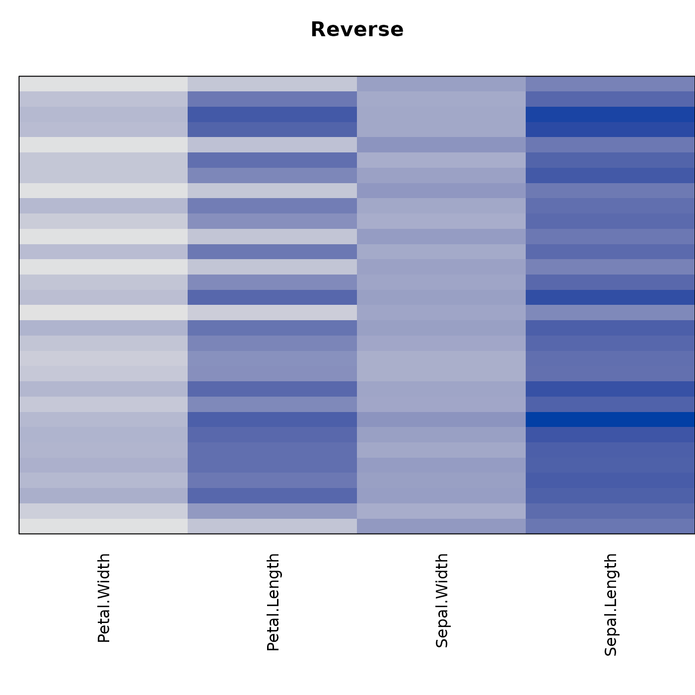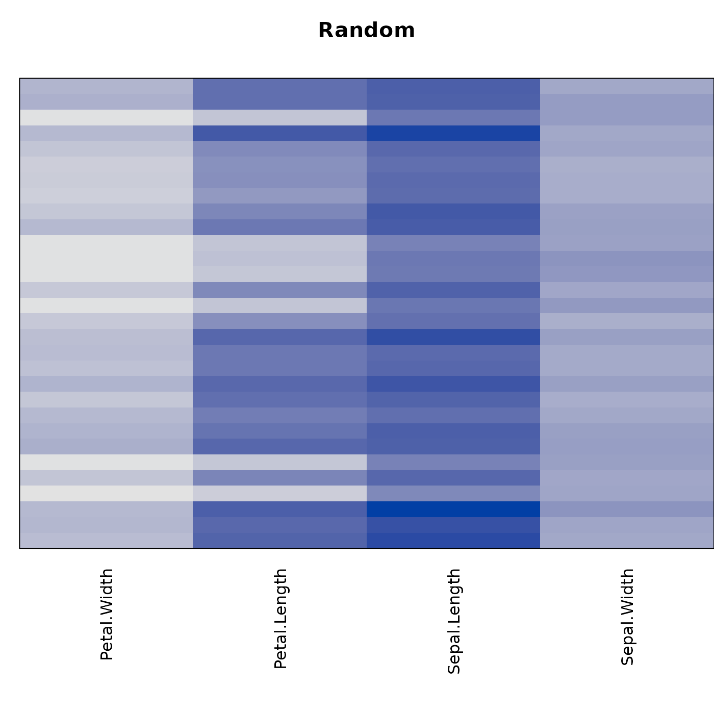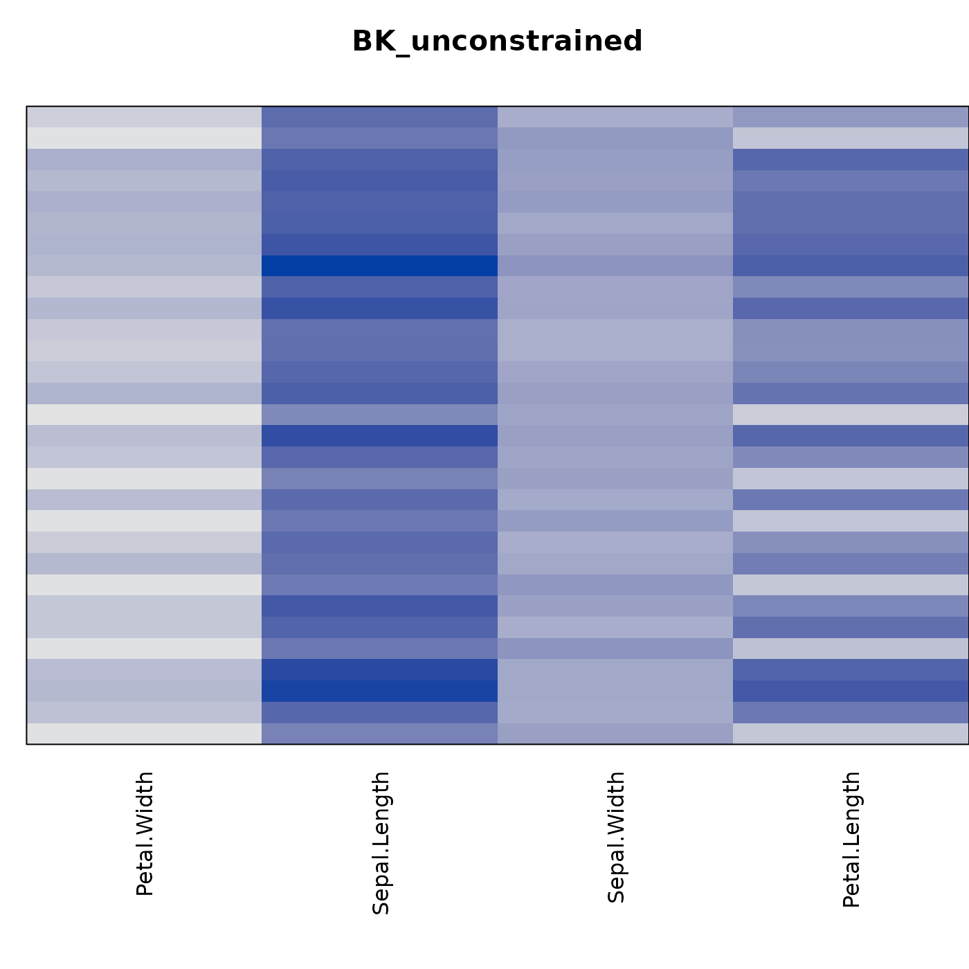
Introduction
This document compares the seriation methods available in the package
seriation using a sample of 30 flowers from the popular
Iris dataset and randomizes the order of the objects.
Distance seriation
We first register more seriation methods. Some of these methods require installing additional packages.
The following methods will be used (a few slow methods are skipped).
methods <- sort(list_seriation_methods("dist"))
methods <- setdiff(methods, c("BBURCG", "BBWRCG", "Enumerate", "GSA", "SGD", "SGLS"))
methods
## [1] "ARSA" "DendSer" "DendSer_ARc" "DendSer_BAR"
## [5] "DendSer_LPL" "DendSer_PL" "GW" "GW_average"
## [9] "GW_complete" "GW_single" "GW_ward" "HC"
## [13] "HC_average" "HC_complete" "HC_single" "HC_ward"
## [17] "Identity" "isoMDS" "MDS" "MDS_angle"
## [21] "MDS_smacof" "OLO" "OLO_average" "OLO_complete"
## [25] "OLO_single" "OLO_ward" "optics" "QAP_2SUM"
## [29] "QAP_BAR" "QAP_Inertia" "QAP_LS" "R2E"
## [33] "Random" "Reverse" "Sammon_mapping" "Spectral"
## [37] "Spectral_norm" "SPIN_NH" "SPIN_STS" "TSP"
## [41] "VAT"Details about the method can be found in the manual
page for seriate().
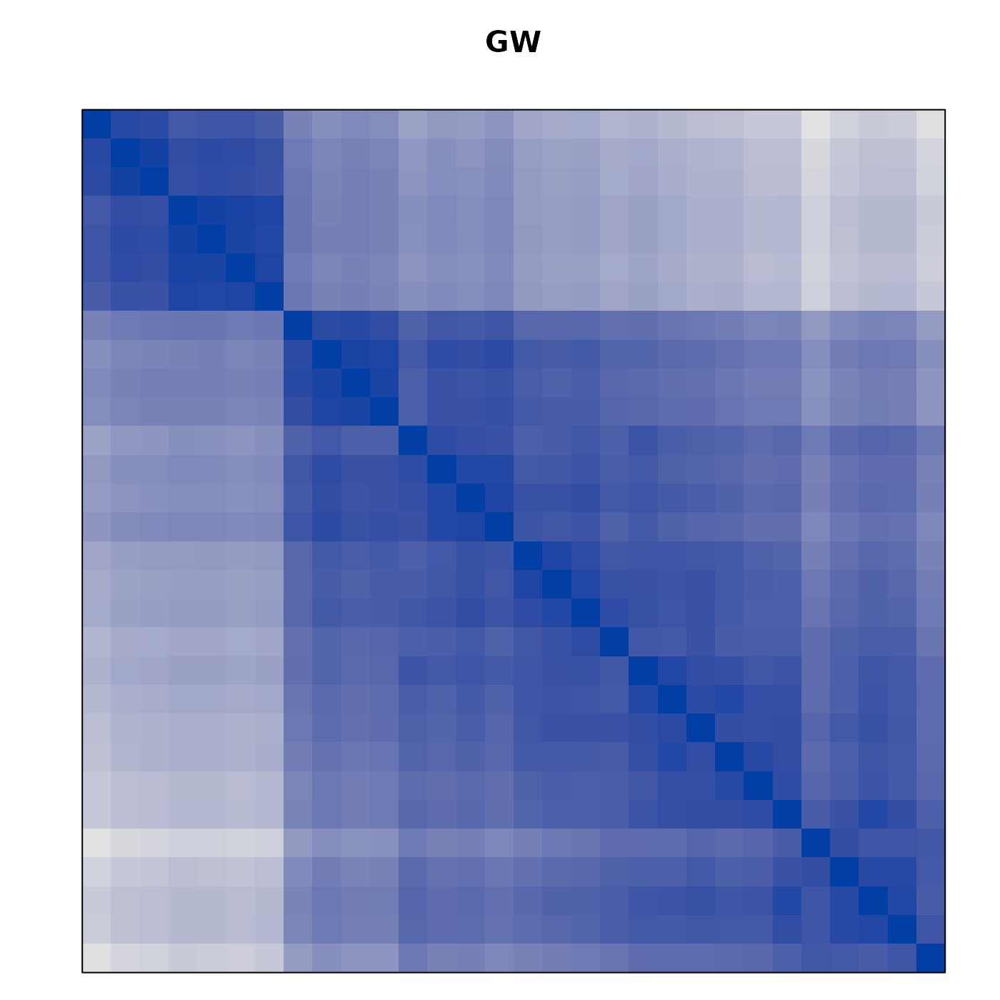
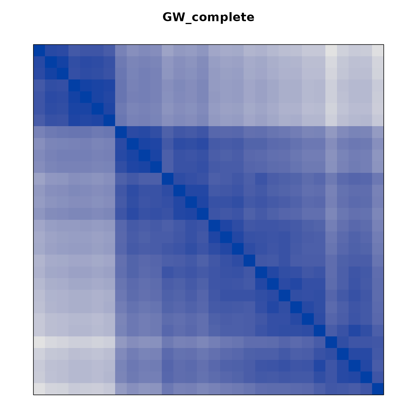
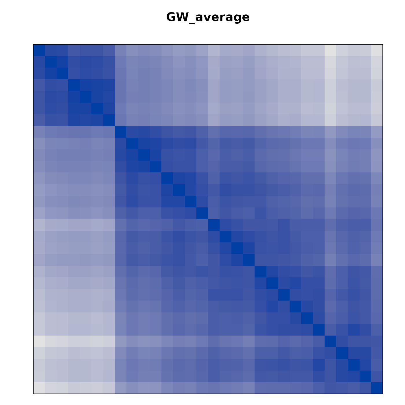
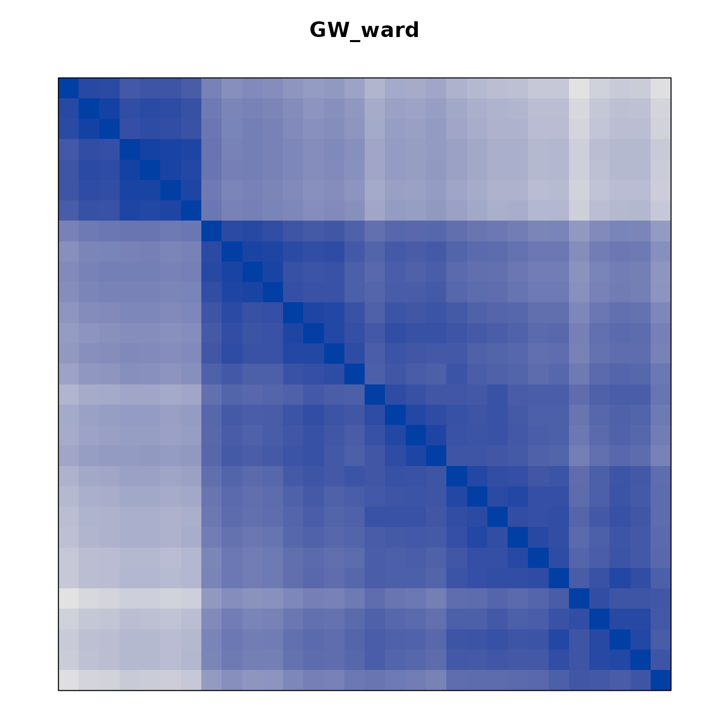
We use a loop to run the function seriate() with each
method and calculate criterion measures which indicate how good the
order is.
orders <- list()
criterion <- list()
for (m in methods) {
  cat(m)
  tm <- system.time(orders[[m]] <- seriate(d, method = m))
  criterion[[m]] <- data.frame(time = tm[1]+tm[2], rbind(criterion(d, orders[[m]])))
  cat(" took", tm[1]+tm[2], "sec.\n")
}
## ARSA took 0.253 sec.
## DendSer took 0.382 sec.
## DendSer_ARc took 0.455 sec.
## DendSer_BAR took 0.387 sec.
## DendSer_LPL took 0.452 sec.
## DendSer_PL took 0.549 sec.
## GW took 0.25 sec.
## GW_average took 0.243 sec.
## GW_complete took 0.243 sec.
## GW_single took 0.231 sec.
## GW_ward took 0.234 sec.
## HC took 0.225 sec.
## HC_average took 0.24 sec.
## HC_complete took 0.232 sec.
## HC_single took 0.22 sec.
## HC_ward took 0.219 sec.
## Identity took 0.234 sec.
## isoMDS took 0.221 sec.
## MDS took 0.226 sec.
## MDS_angle took 0.23 sec.
## MDS_smacof took 0.223 sec.
## OLO took 0.24 sec.
## OLO_average took 0.227 sec.
## OLO_complete took 0.238 sec.
## OLO_single took 0.222 sec.
## OLO_ward took 0.222 sec.
## optics took 0.231 sec.
## QAP_2SUM took 0.231 sec.
## QAP_BAR took 0.22 sec.
## QAP_Inertia took 0.225 sec.
## QAP_LS took 0.214 sec.
## R2E took 0.21 sec.
## Random took 0.225 sec.
## Reverse took 0.24 sec.
## Sammon_mapping took 0.239 sec.
## Spectral took 0.238 sec.
## Spectral_norm took 0.226 sec.
## SPIN_NH took 0.264 sec.
## SPIN_STS took 0.227 sec.
## TSP took 0.233 sec.
## VAT took 0.218 sec.
criterion <- do.call(rbind, criterion)We align the seriation orders. The reason is that an order 1, 2, 3
and 3, 2, 1 are equivalent and just an artifact of the algorithm.
Aligning will reverse some orders so they are better aligned. Then we
sort the orders from best to worst according to a popular seriation
criterion measure called Gradient_weighted.
orders <- ser_align(orders)
best_to_worse <- order(criterion[["Gradient_weighted"]], decreasing = TRUE)

orders <- orders[best_to_worse]
criterion <- criterion[best_to_worse, ]
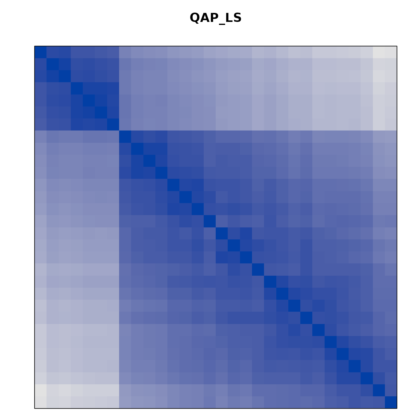
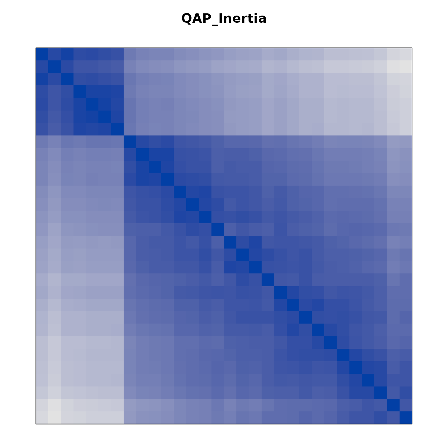
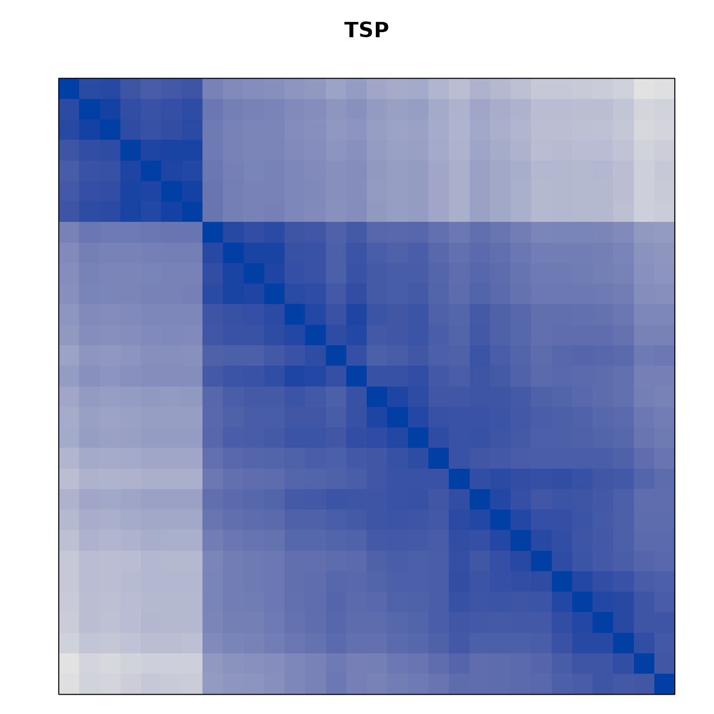
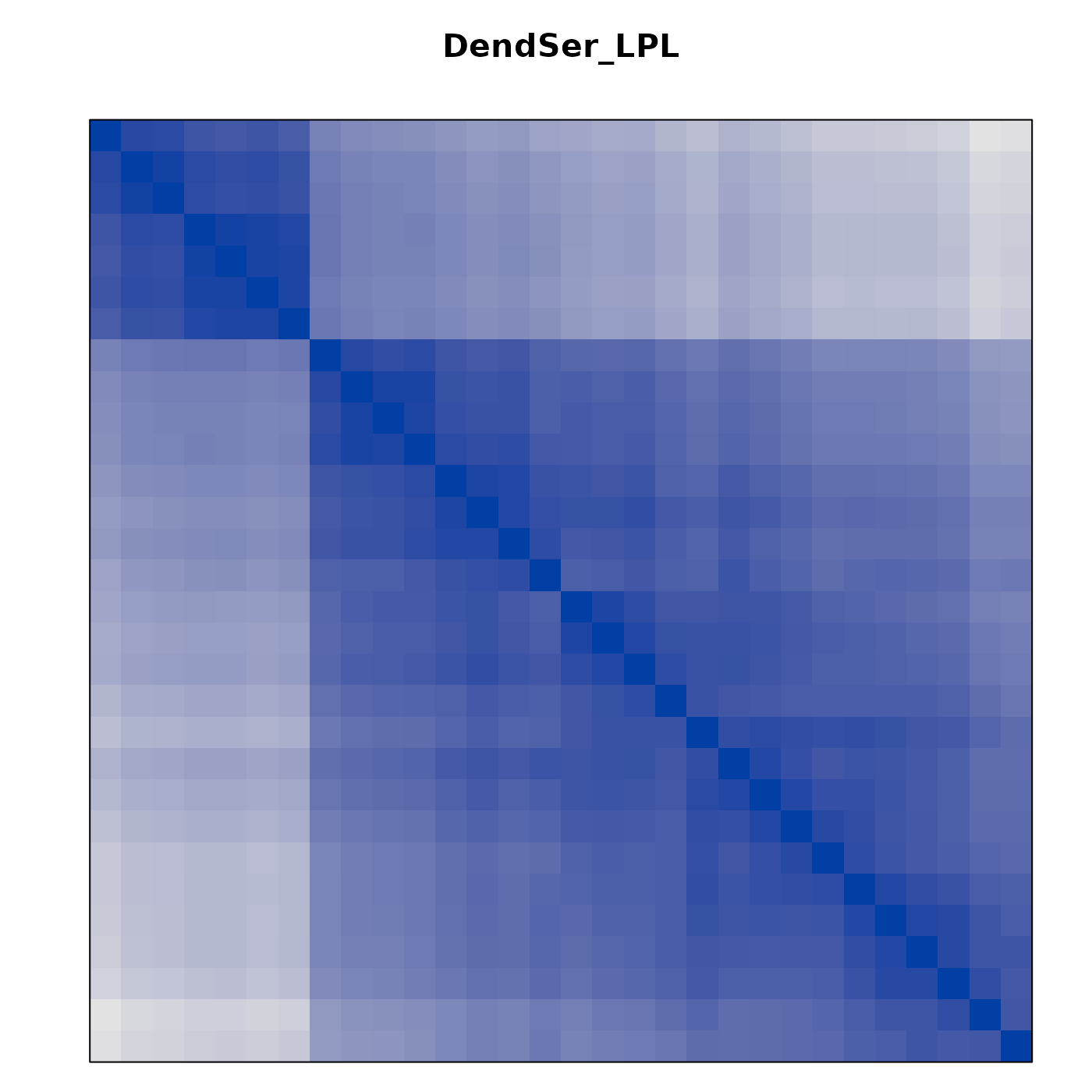
Comparison between methods
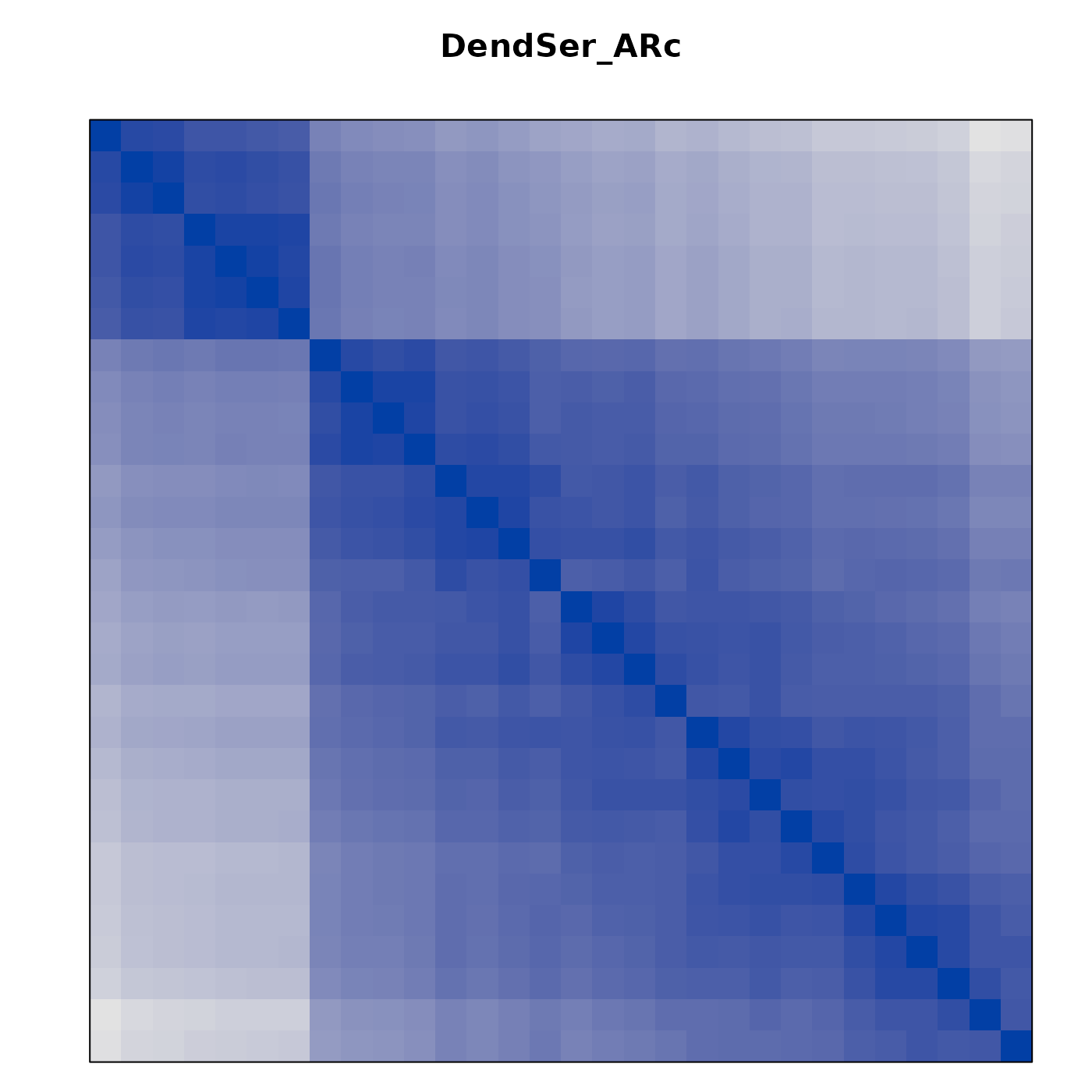
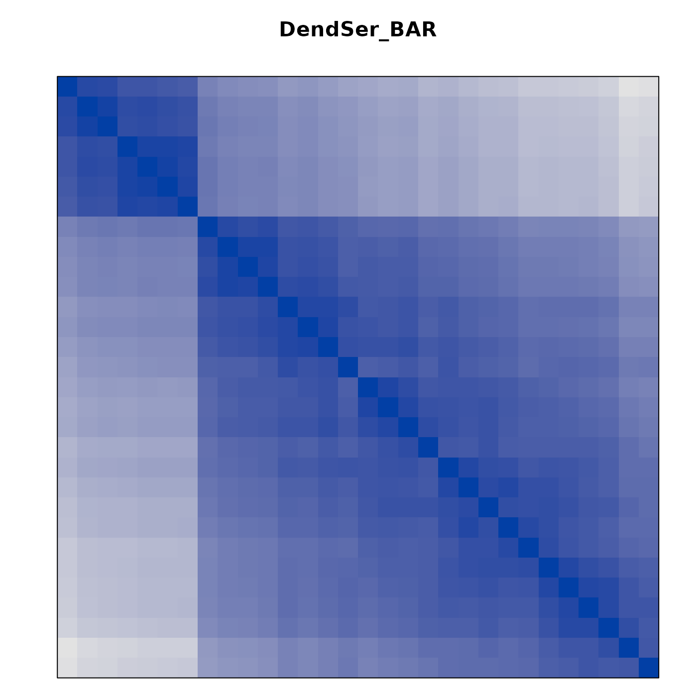
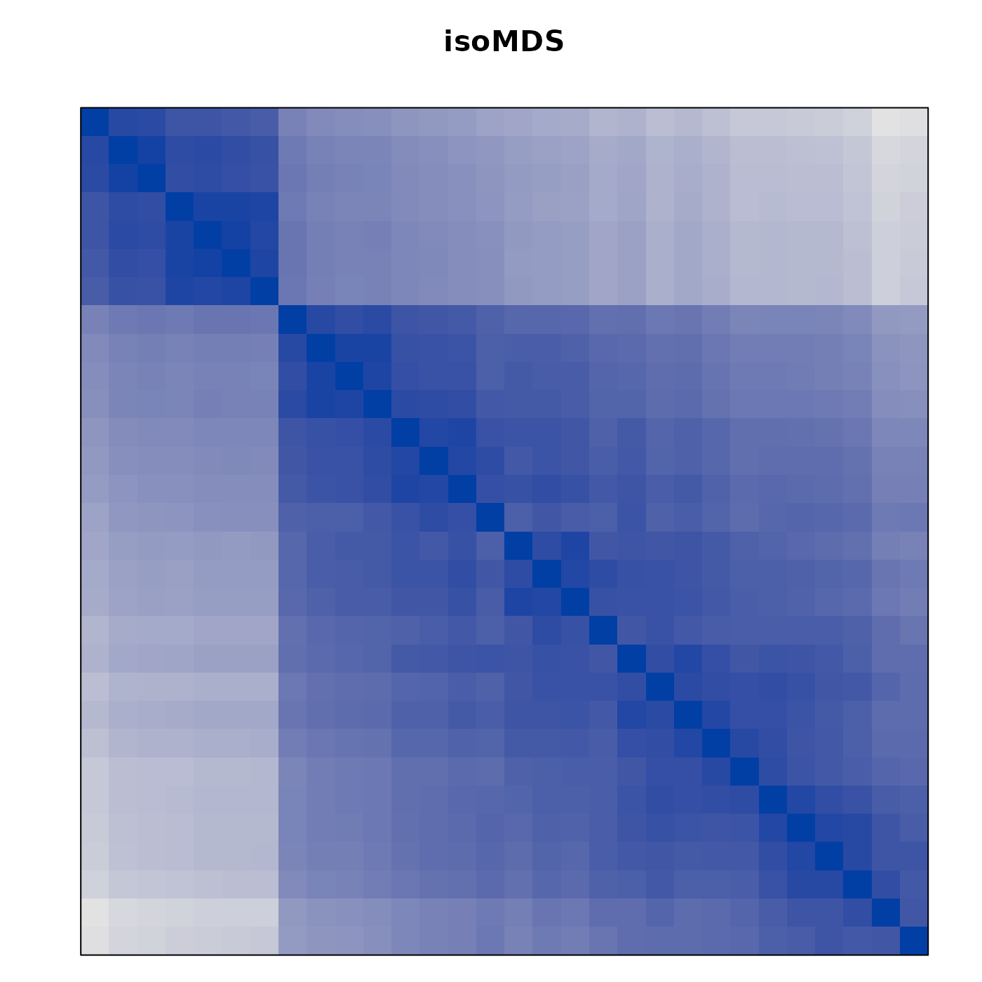
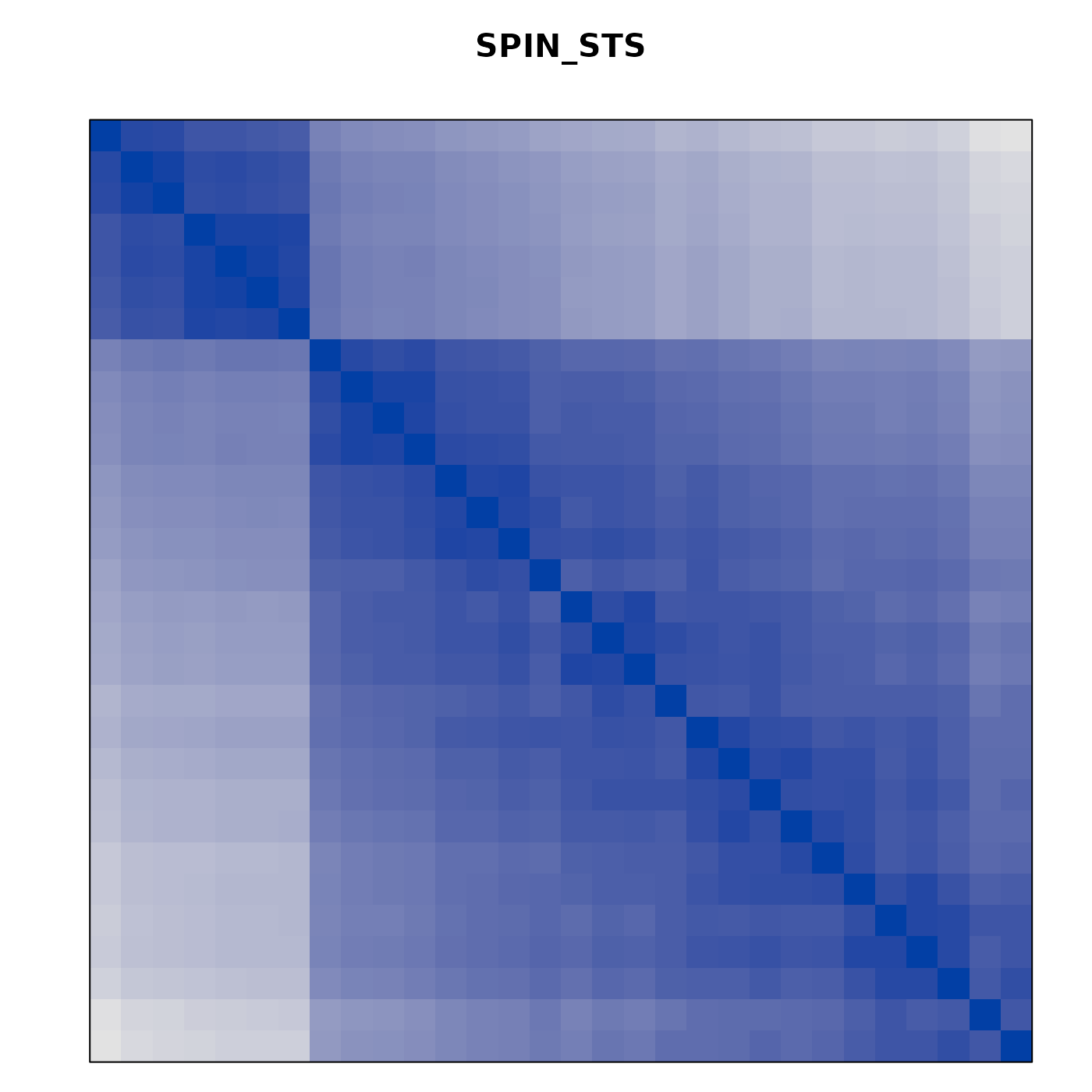
We can compare the seriation methods by how similar the orders are that they produce (measured using Spearman). The following code calculates distances between orders and then performs hierarchical clustering.

The reordered dendrogram clearly shows a group of methods based on hierarchical clustering focused on path length and another group that tries to optimize the other seriation measures.
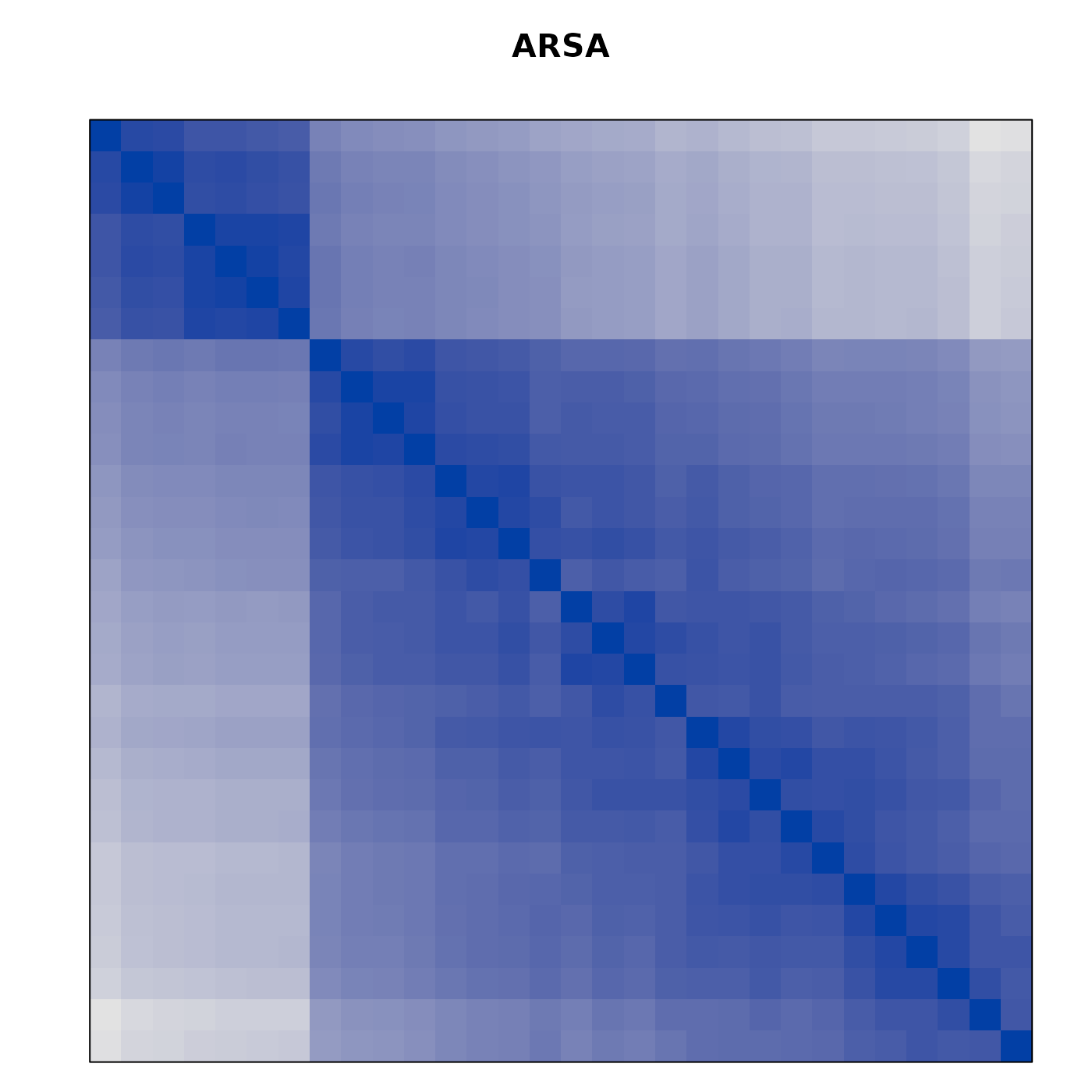
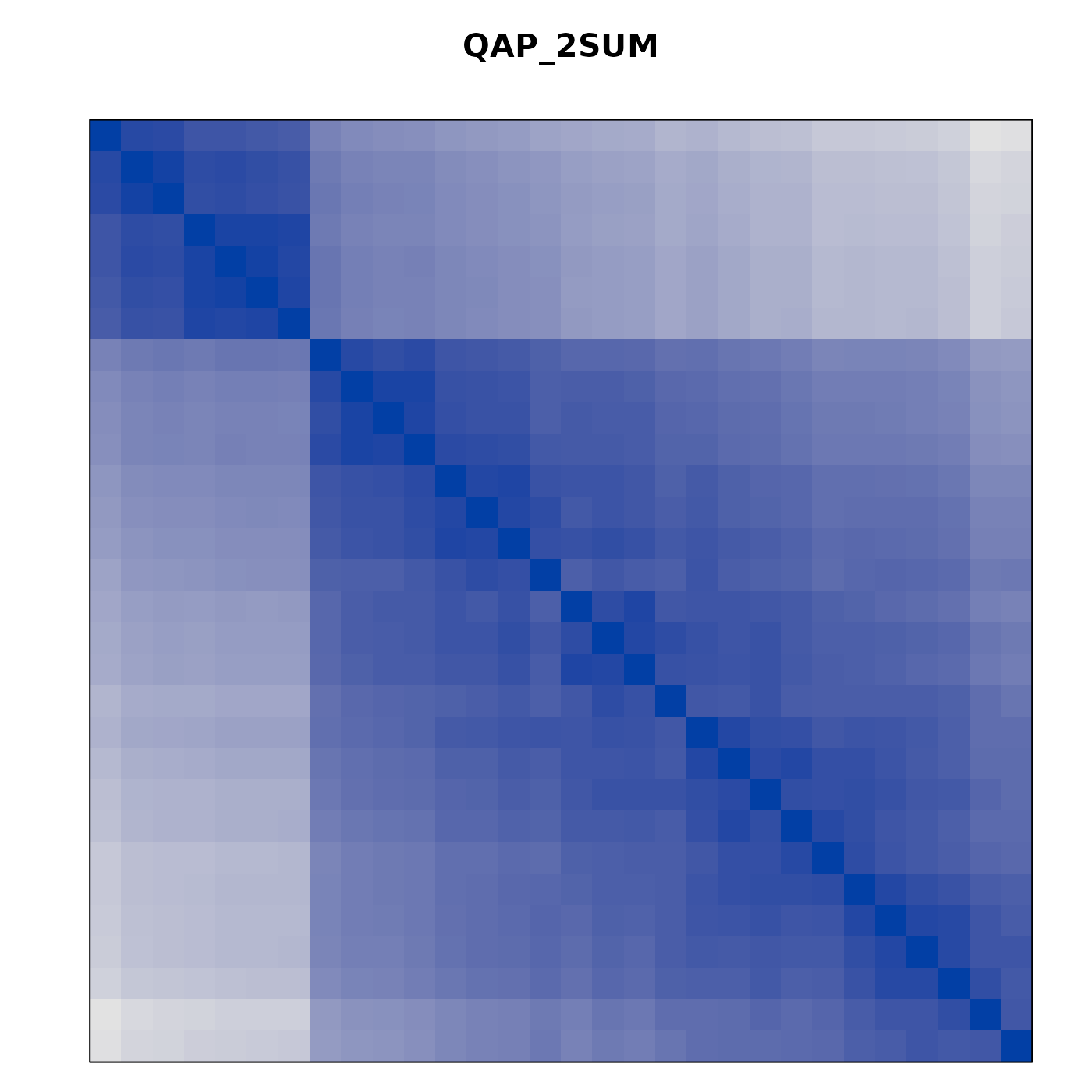
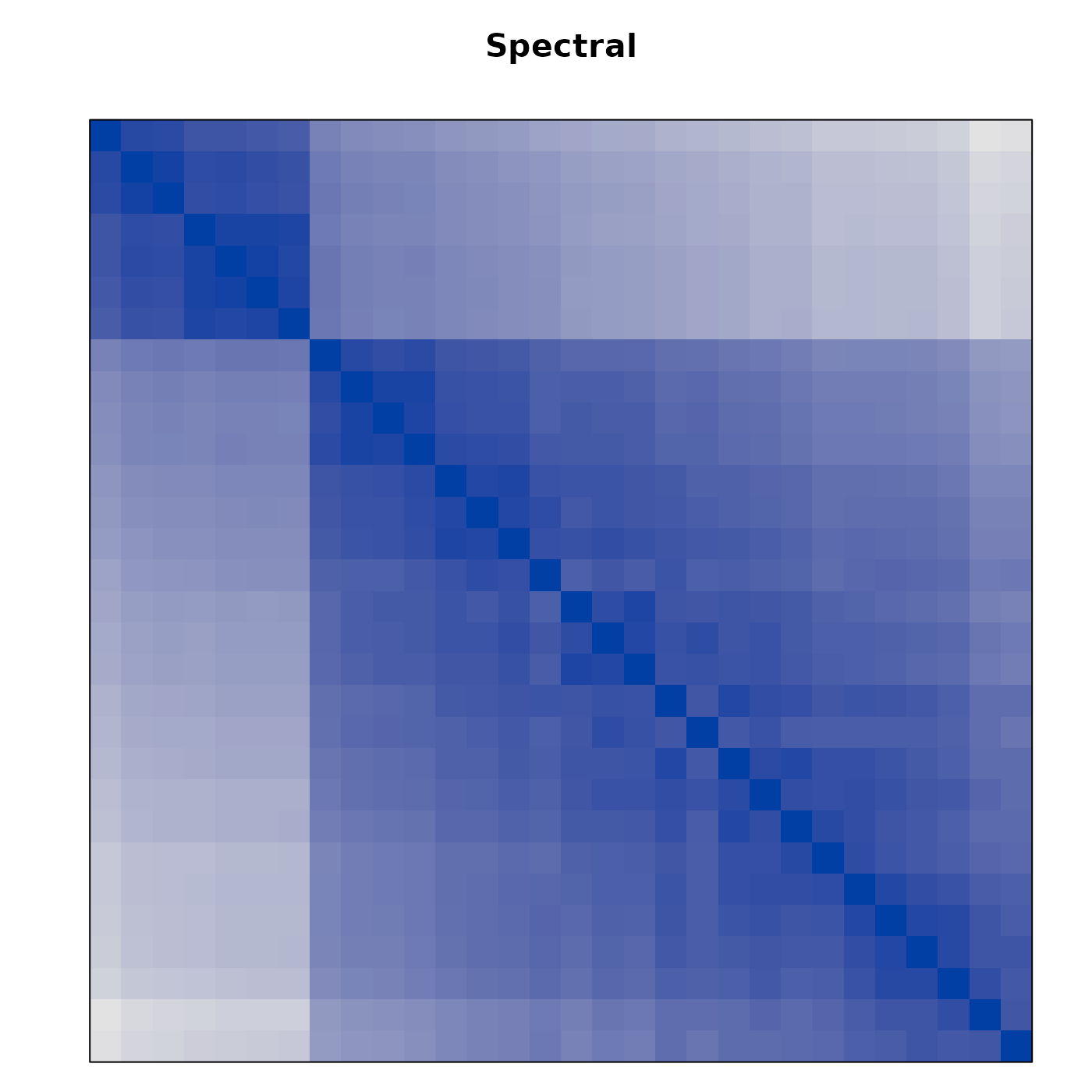
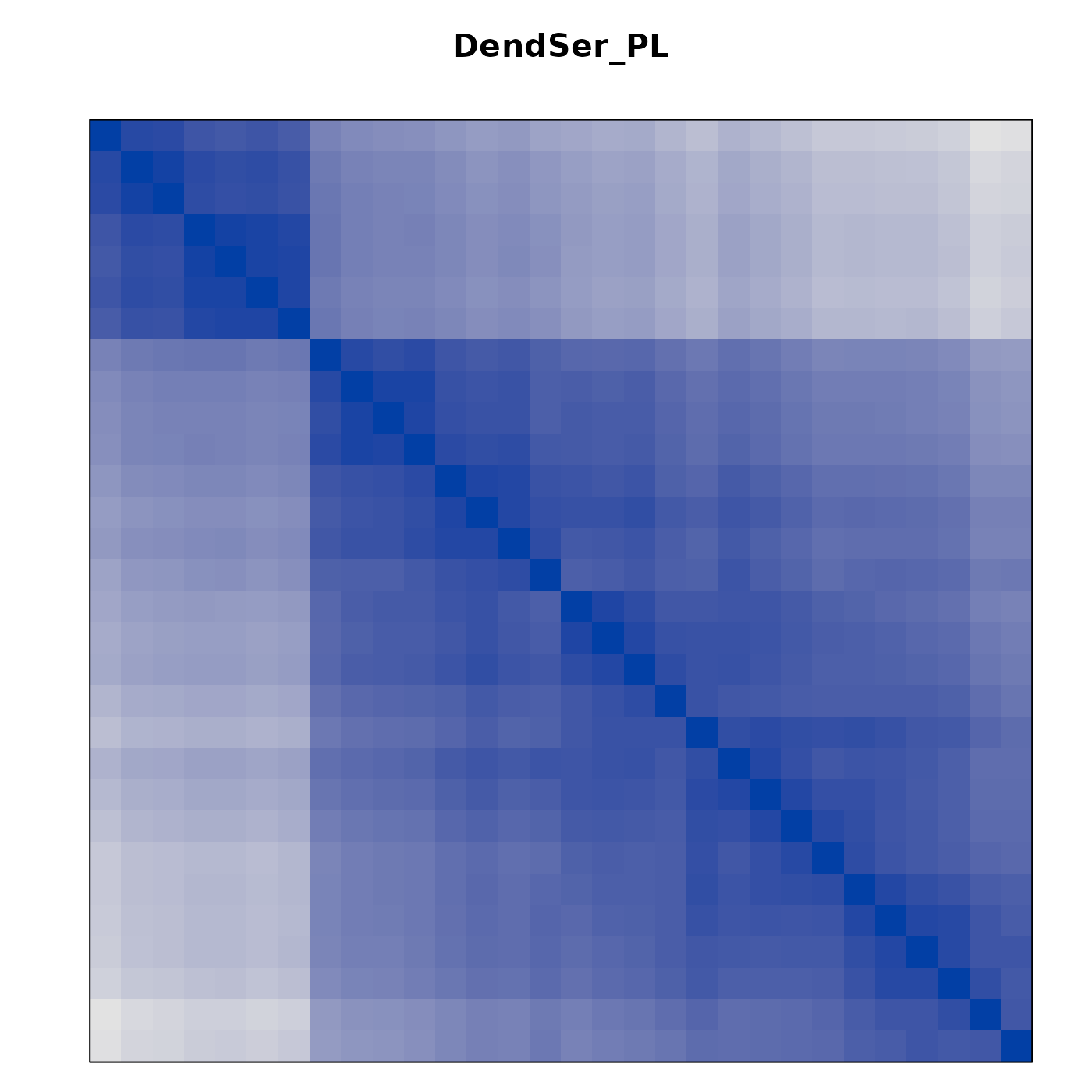
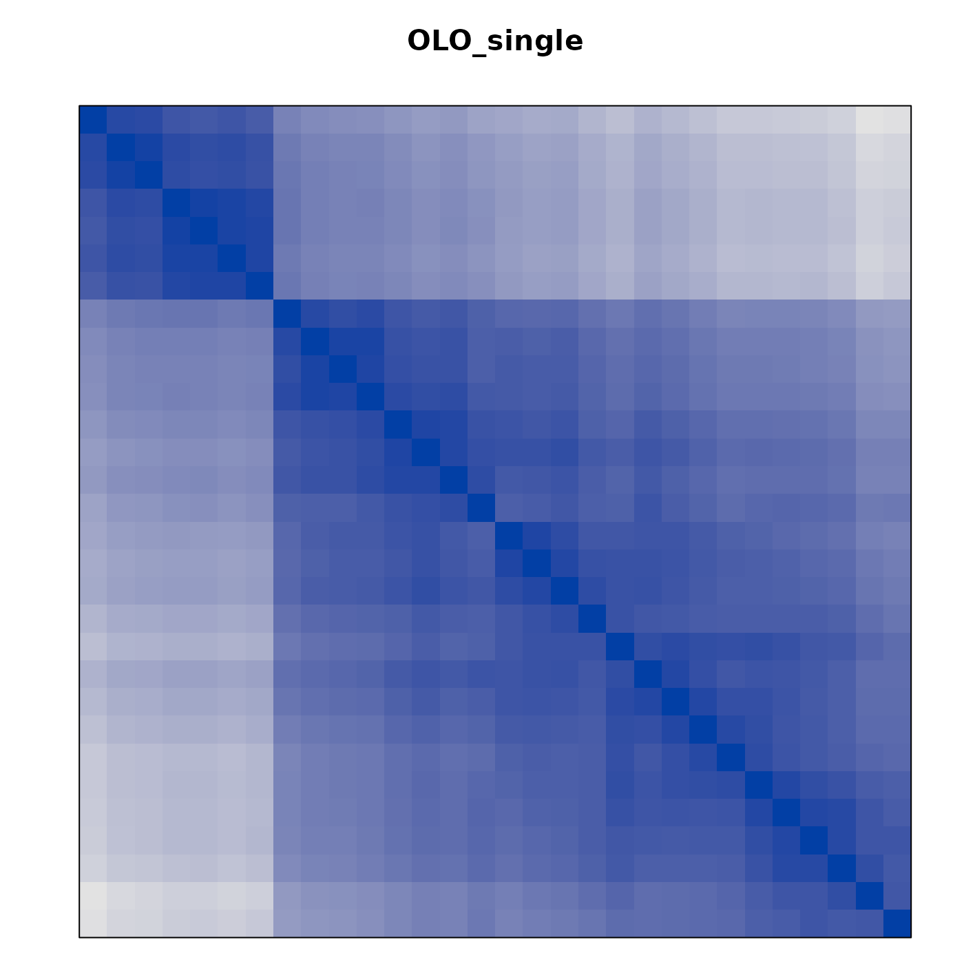
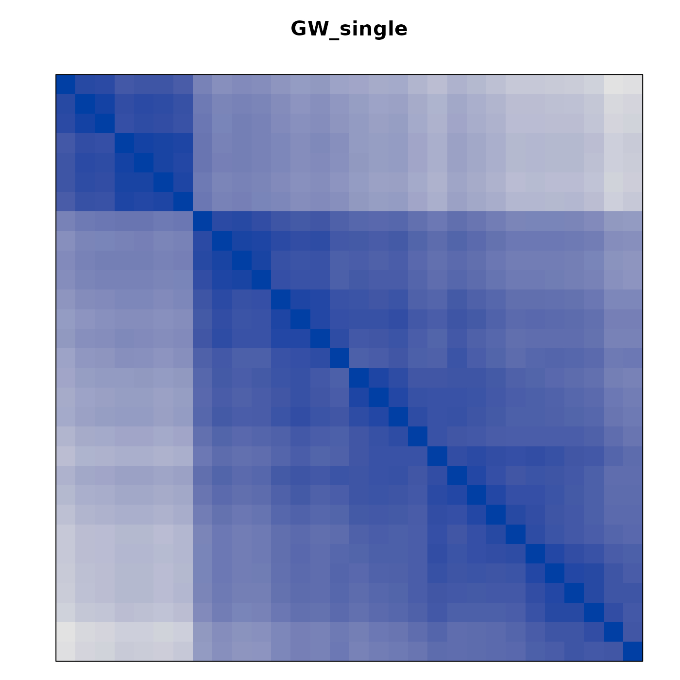
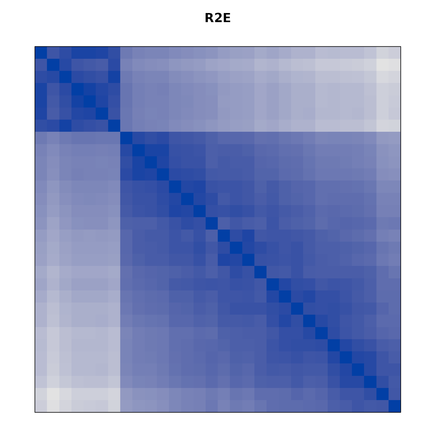
Here is a table to compare the seriation methods on different
criterion measures. Use the interactive table to sort the methods given
different measures. Note that some are maximized and some should be
minimized. Details about the measures can be found in the manual
page for criterion().
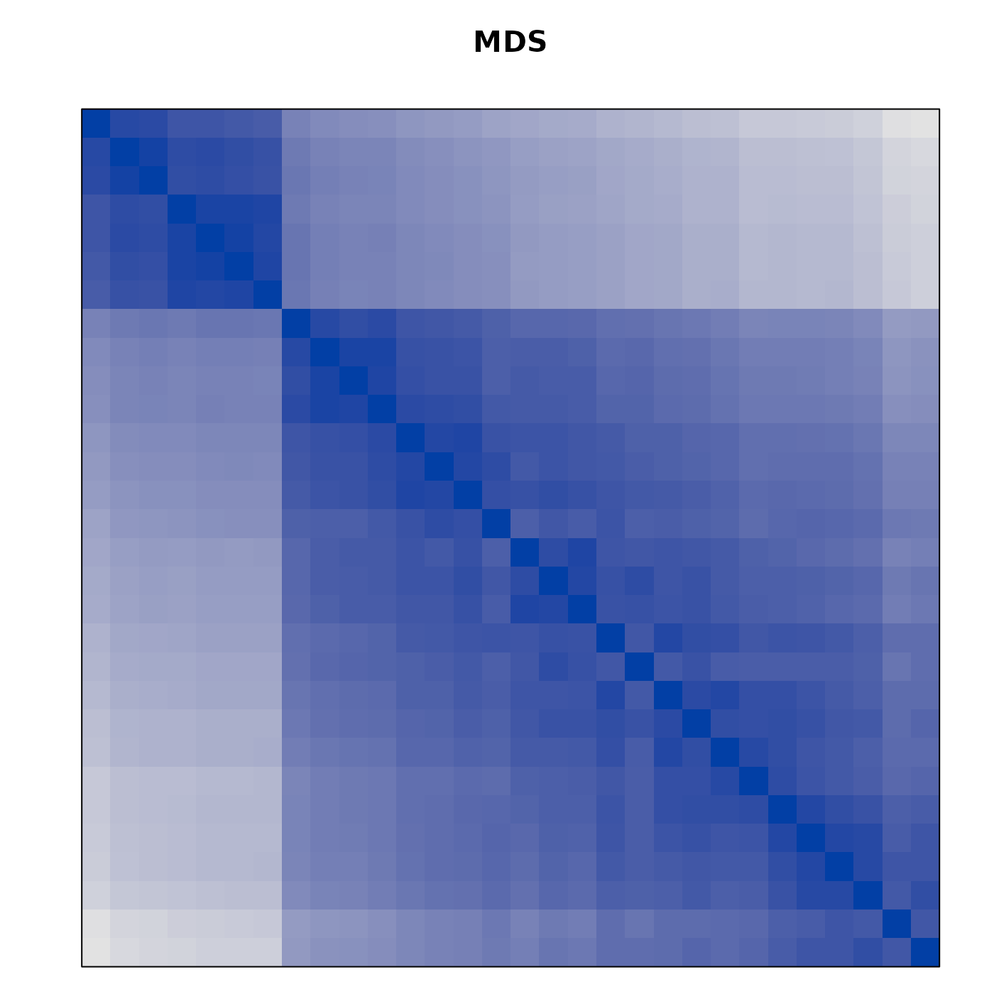
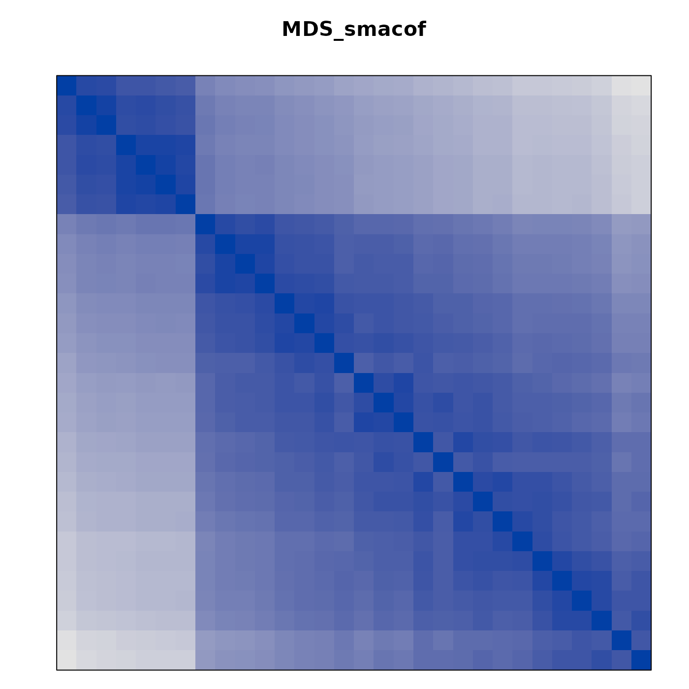
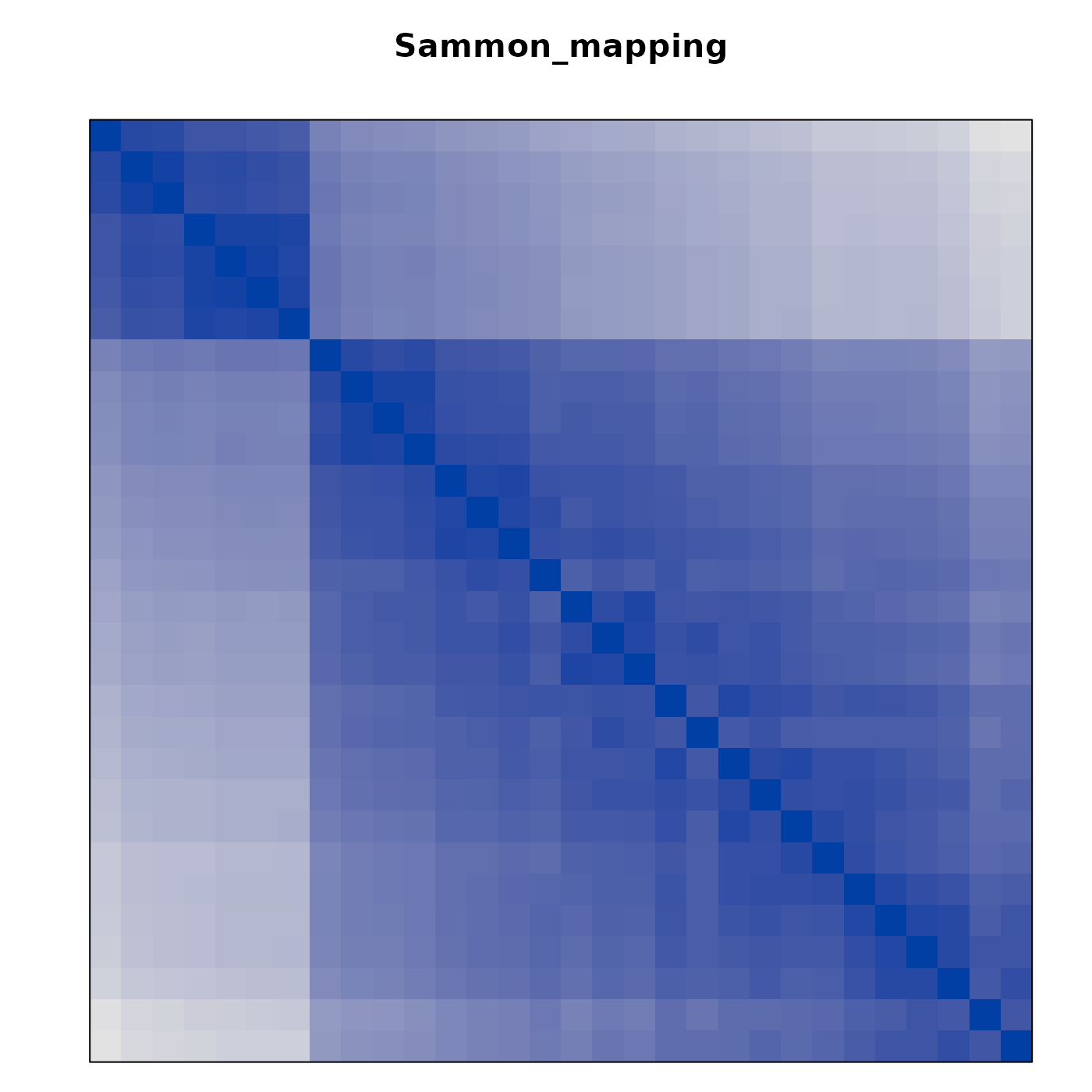
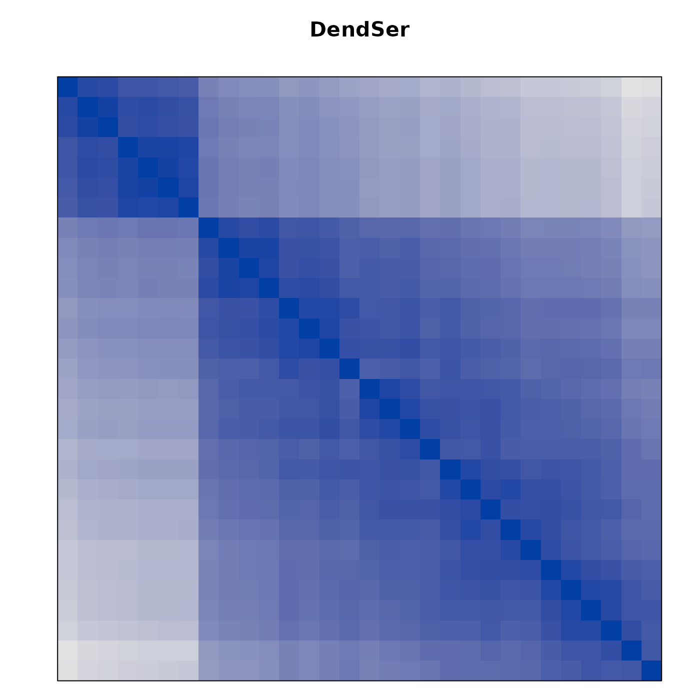
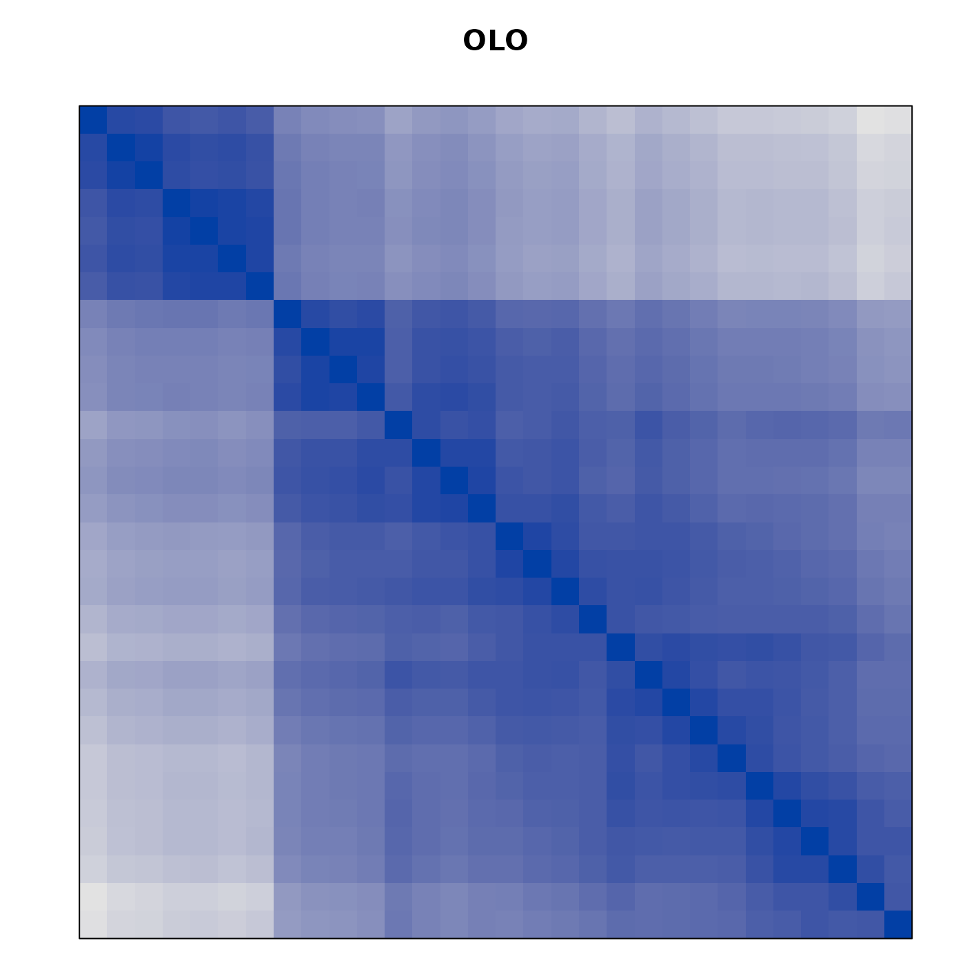
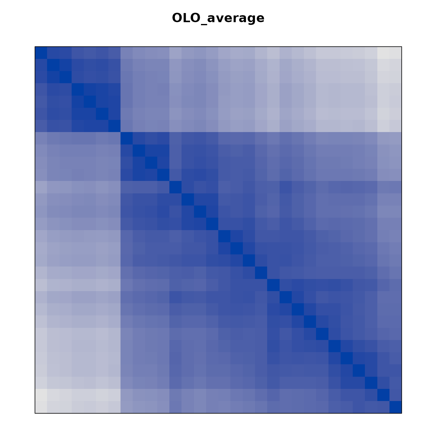
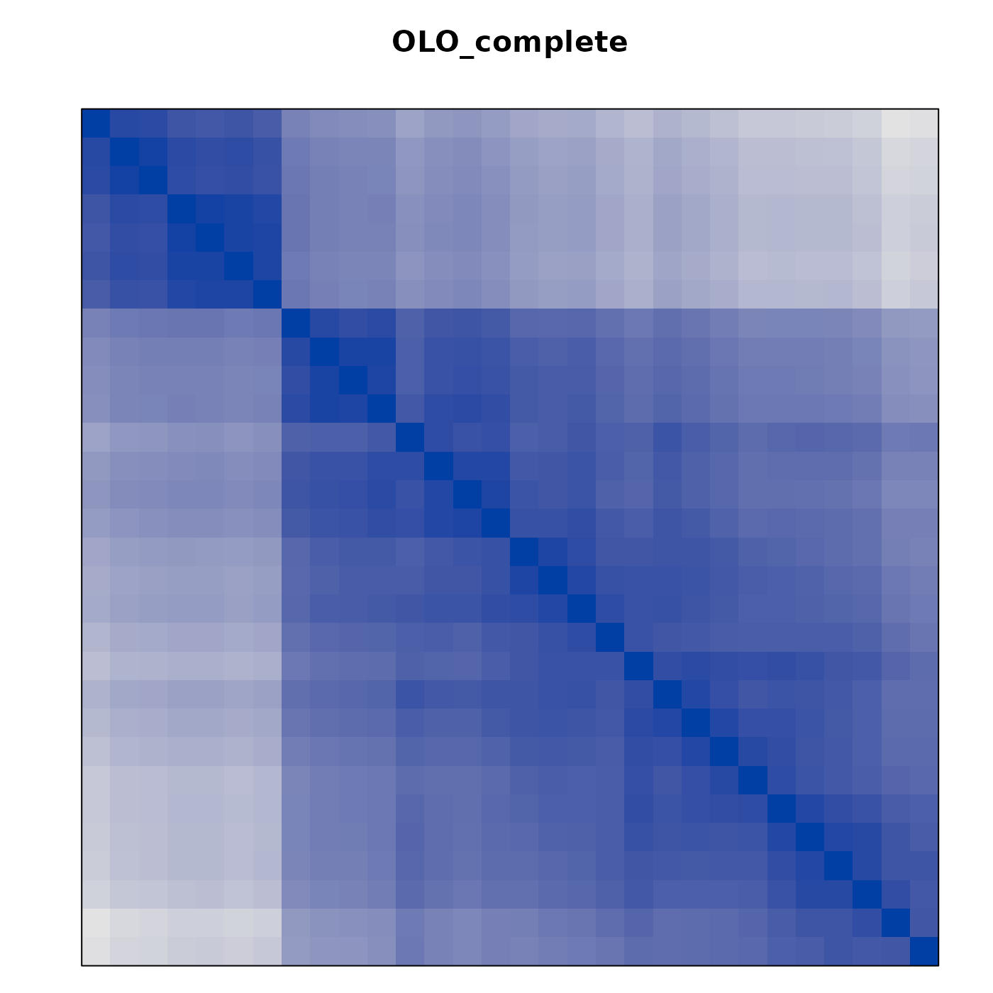
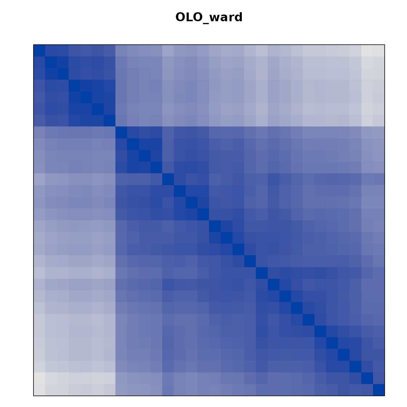
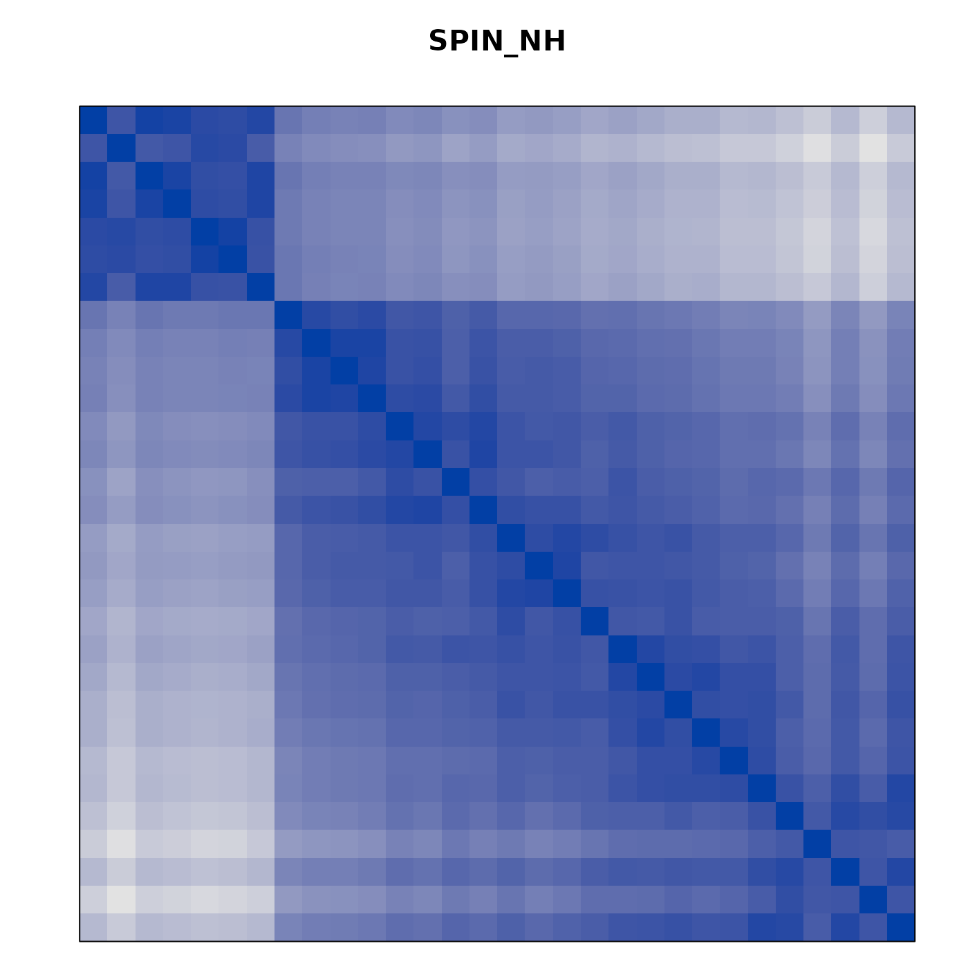
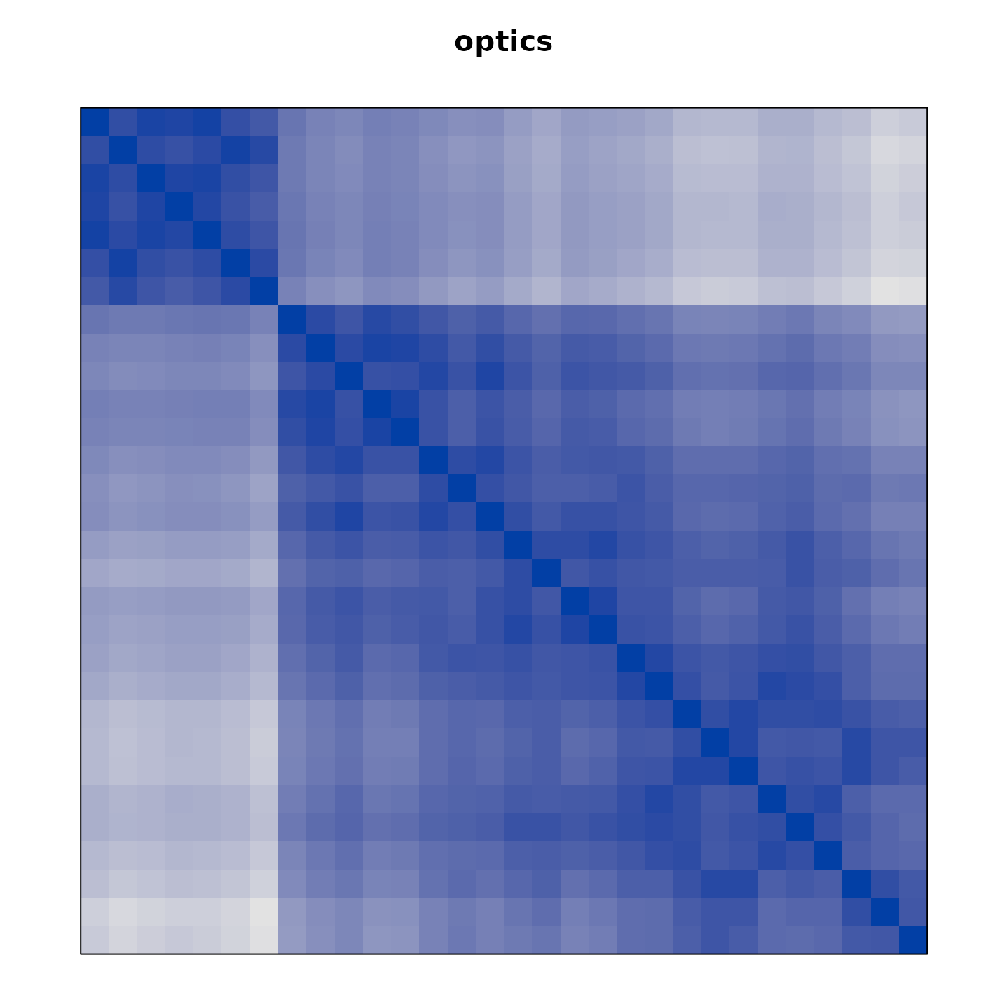
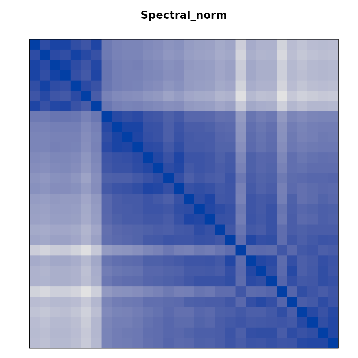
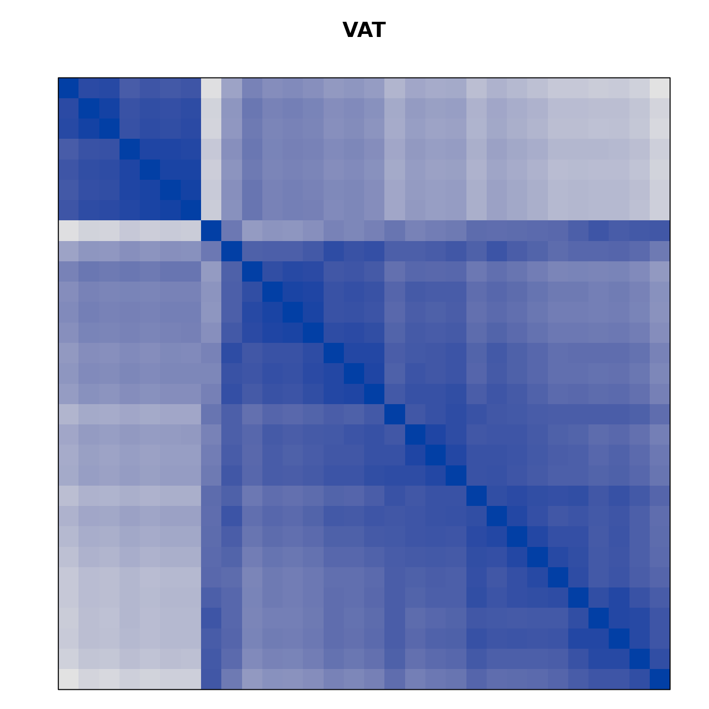
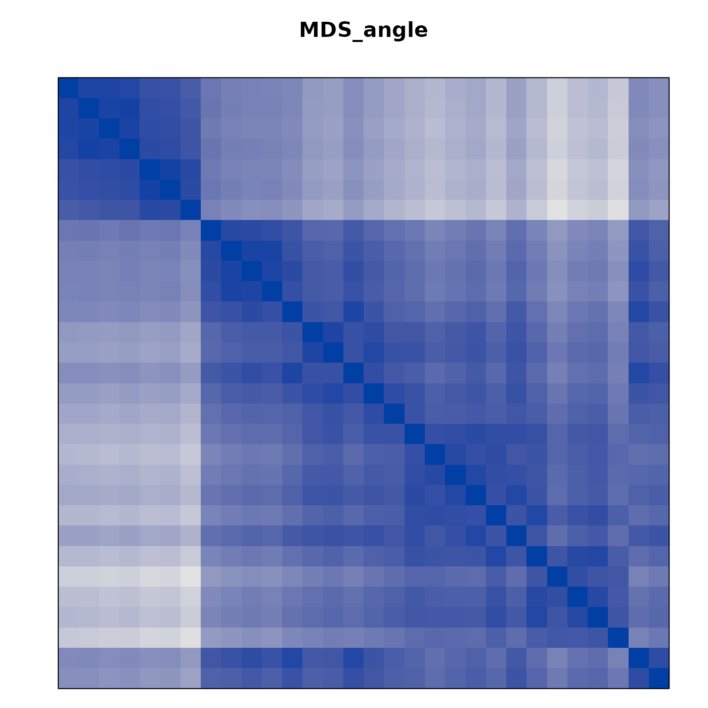
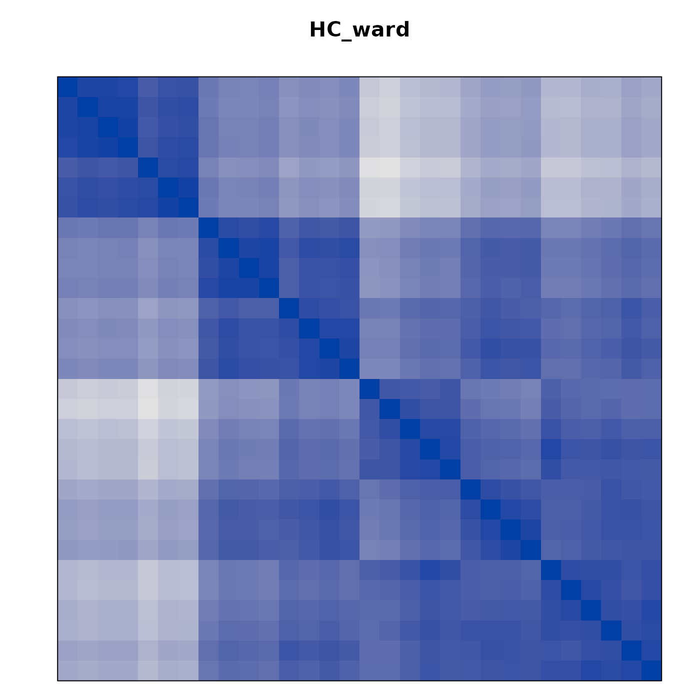
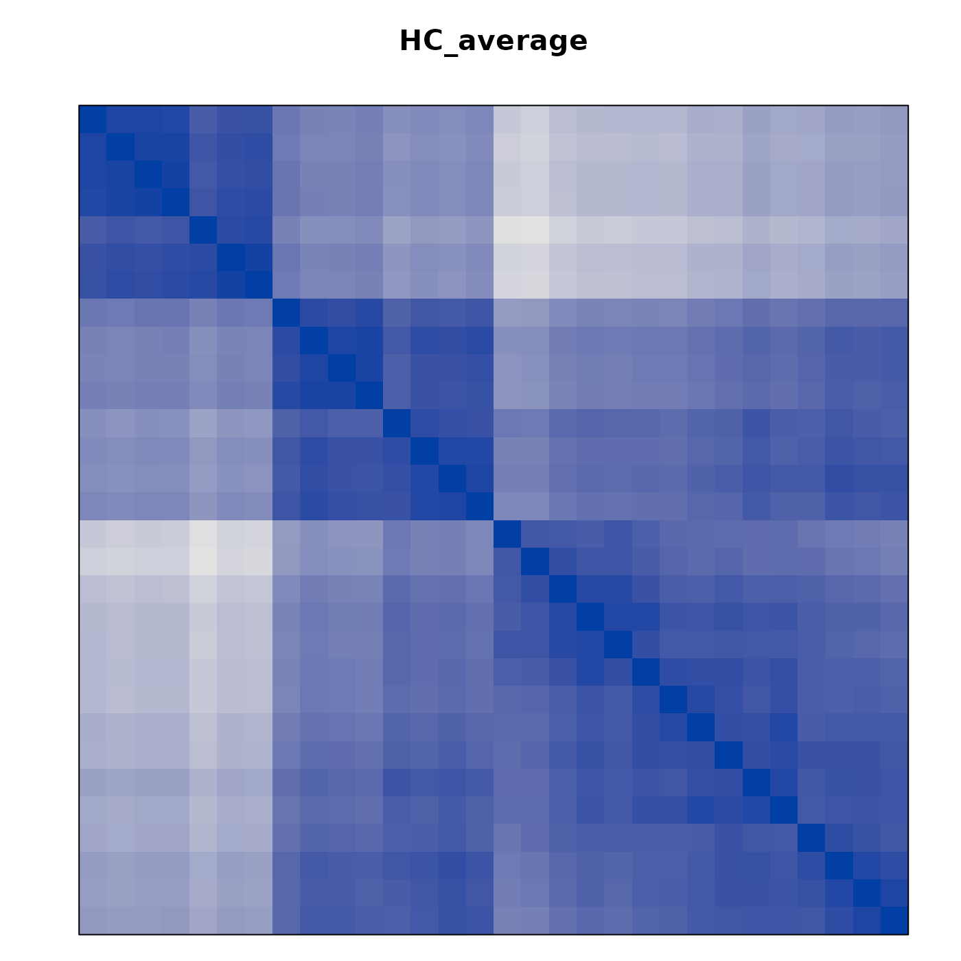
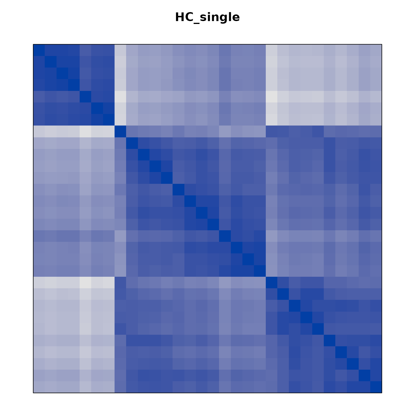
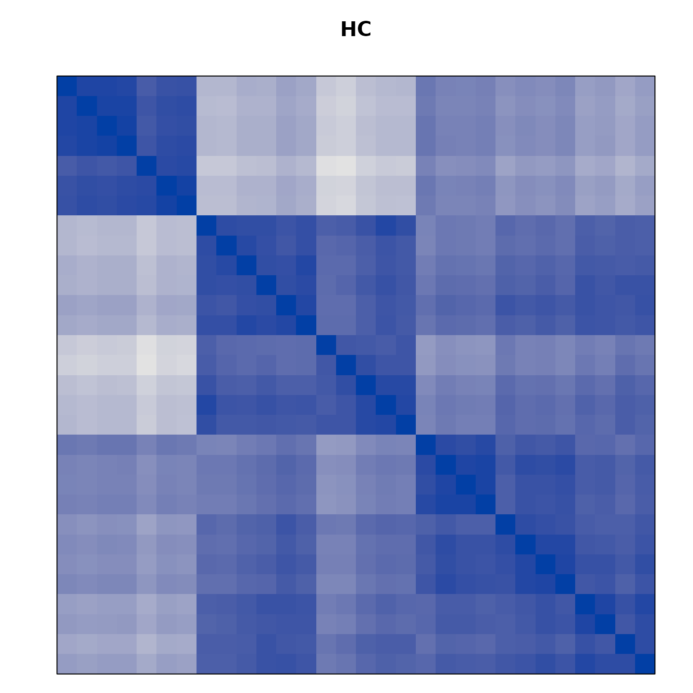
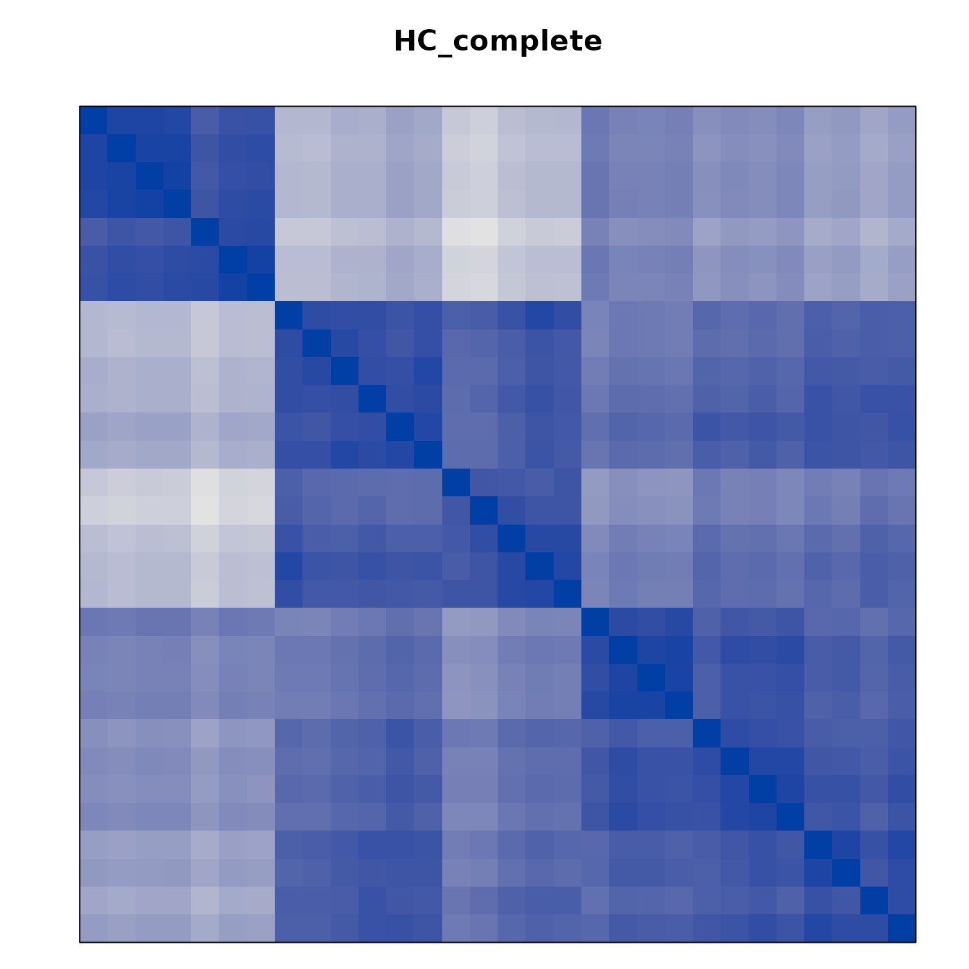
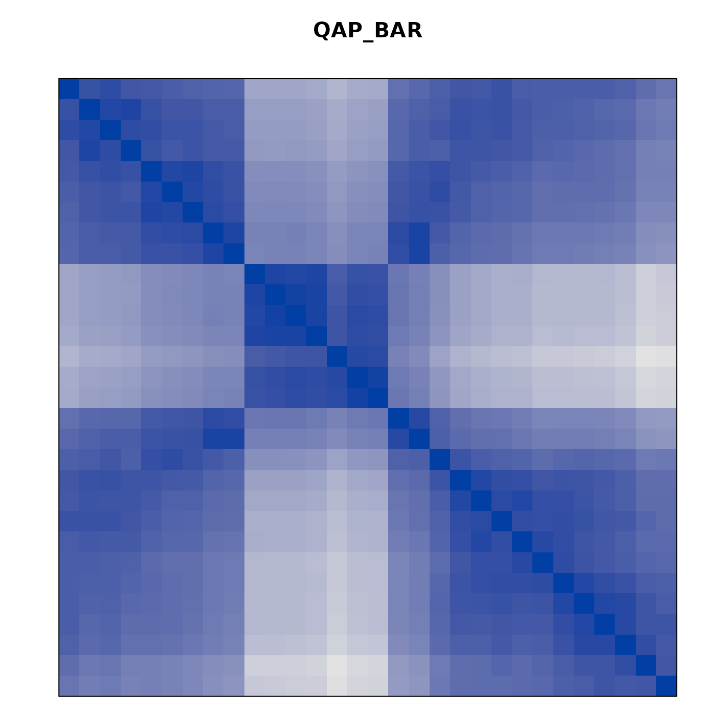
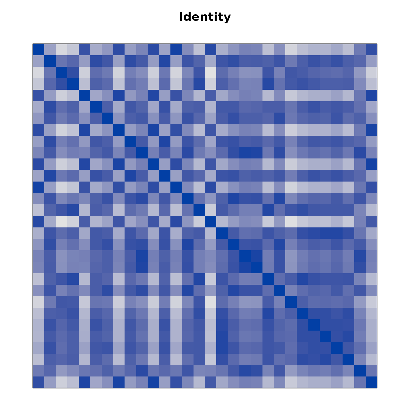
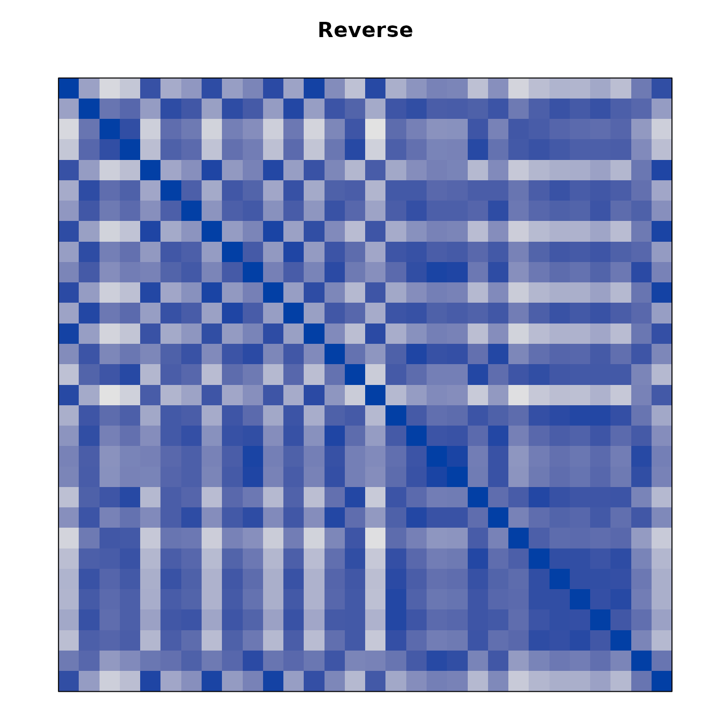
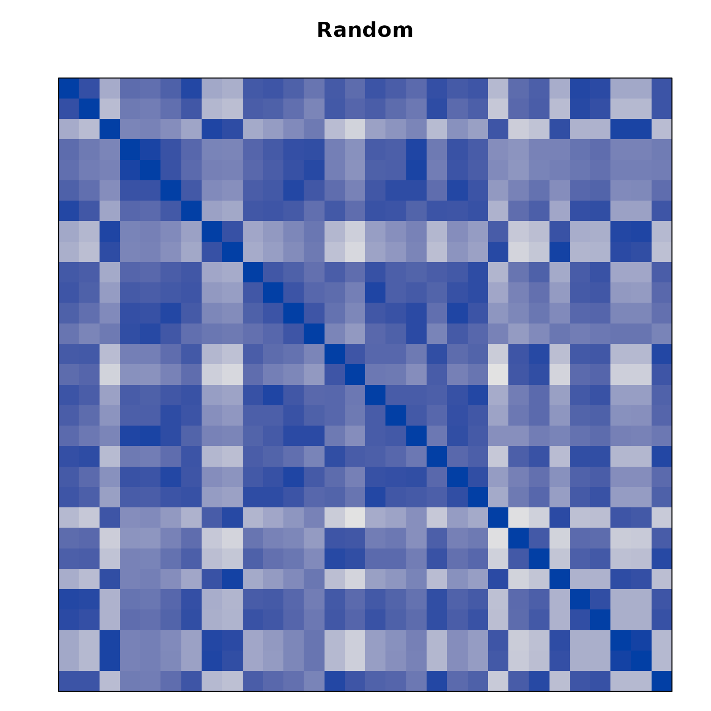
Matrix seriation
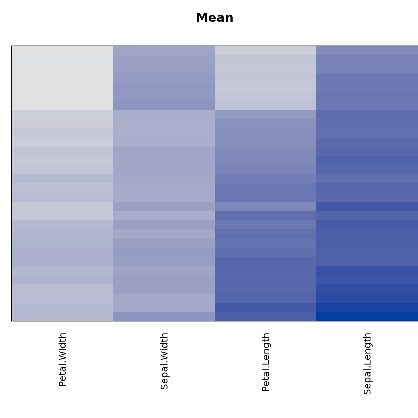
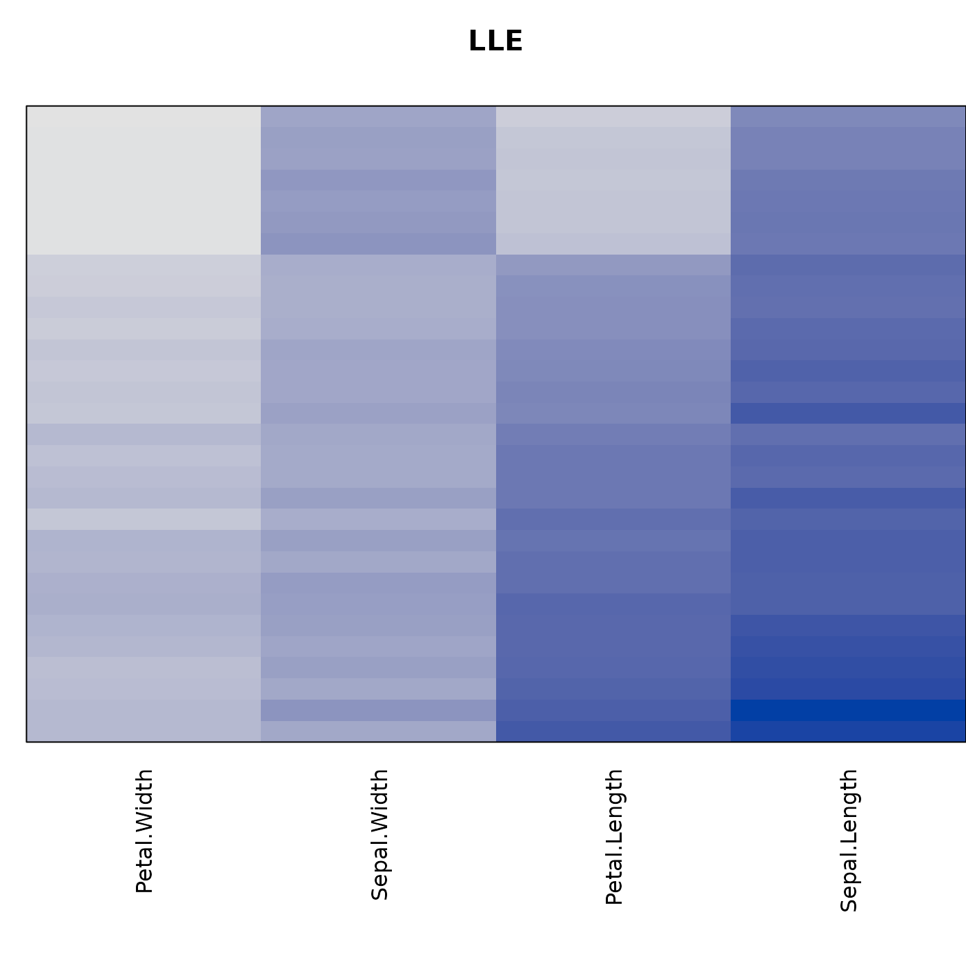
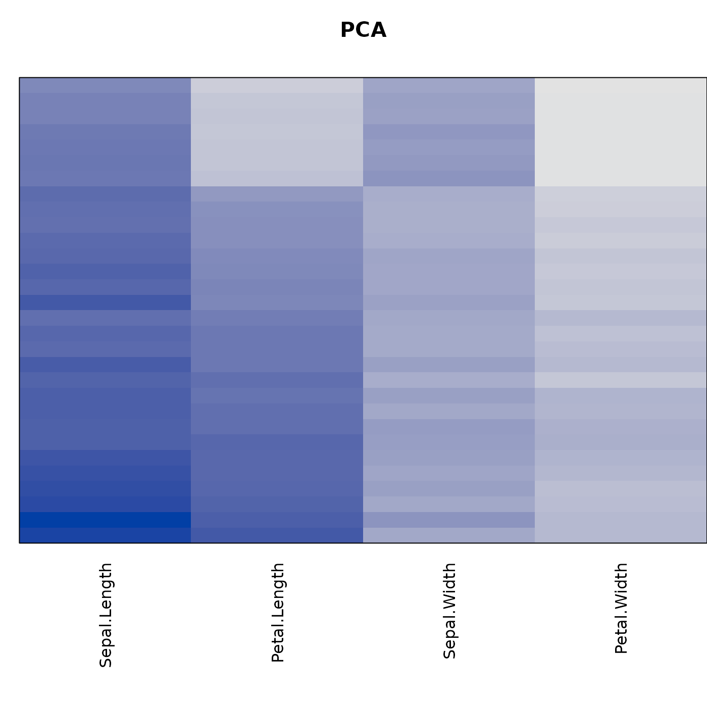
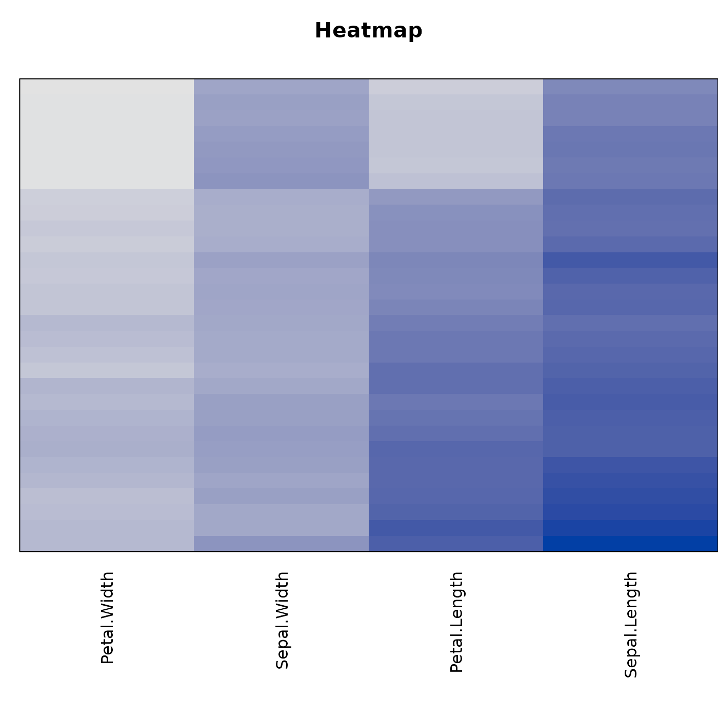
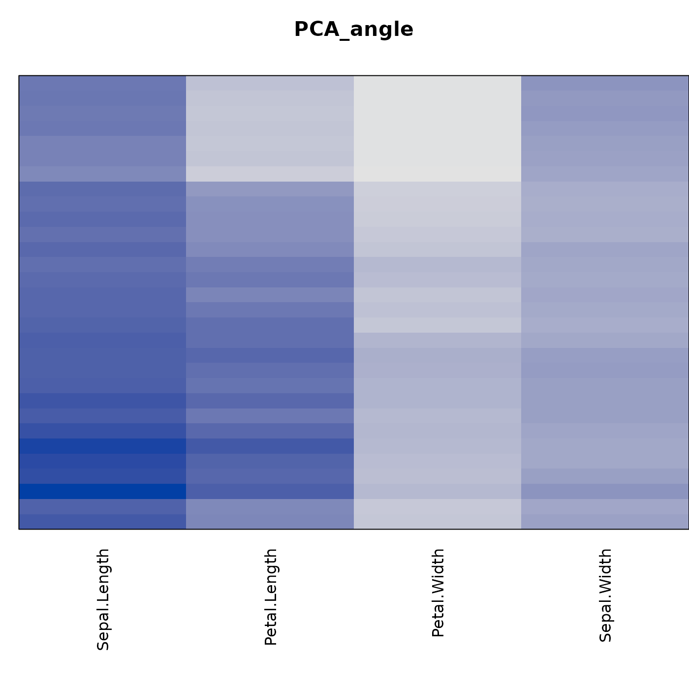
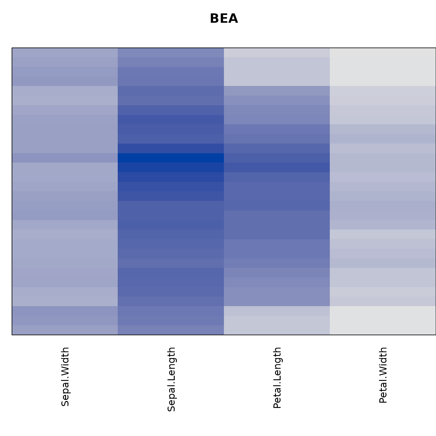
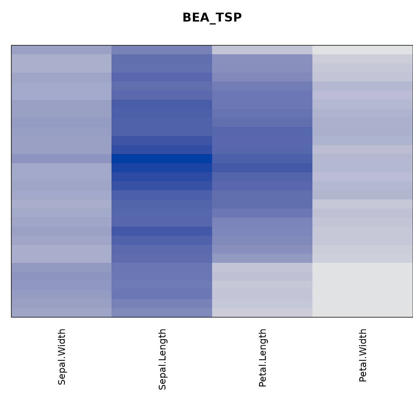
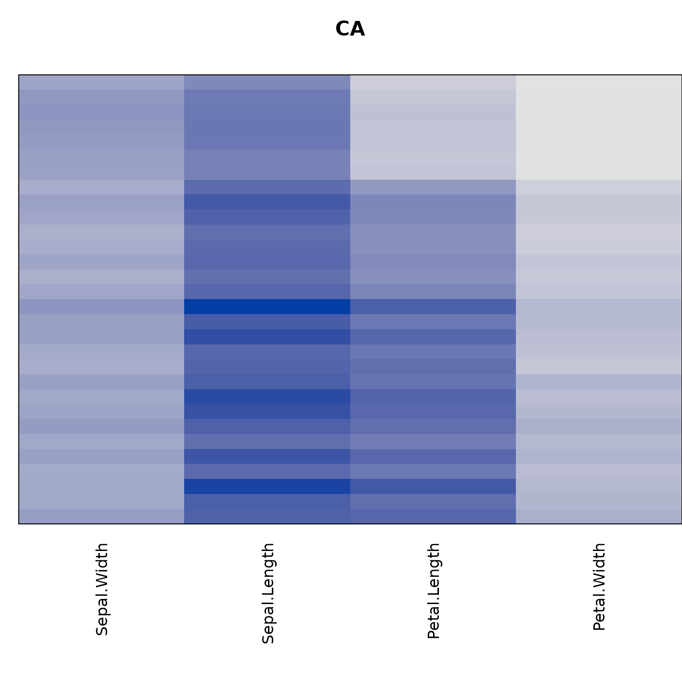
Matrix seriation reorders rows and columns of a data matrix. We perform the same steps as for distances in the previous section.
methods <- sort(list_seriation_methods("matrix"))

# AOE if for correlation matrices only
methods <- setdiff(methods, c("AOE"))
methods
## [1] "BEA" "BEA_TSP" "BK_unconstrained" "CA"
## [5] "Heatmap" "Identity" "LLE" "Mean"
## [9] "PCA" "PCA_angle" "Random" "Reverse"Performing seriation.
orders <- list()
criterion <- list()
for (m in methods) {
  cat(m)
  tm <- system.time(orders[[m]] <- seriate(x, method = m))
  criterion[[m]] <- data.frame(time = tm[1]+tm[2], rbind(criterion(x, orders[[m]])))
  cat(" took", tm[1]+tm[2], "sec.\n")
}
## BEA took 0.749 sec.
## BEA_TSP took 0.764 sec.
## BK_unconstrained took 0.253 sec.
## CA took 0.264 sec.
## Heatmap took 0.767 sec.
## Identity took 0.256 sec.
## LLE took 0.261 sec.
## Mean took 0.256 sec.
## PCA took 0.246 sec.
## PCA_angle took 0.258 sec.
## Random took 0.249 sec.
## Reverse took 0.26 sec.
criterion <- do.call(rbind, criterion)Visualize the results
best_to_worse <- order(criterion[["Moore_stress"]], decreasing = FALSE)

orders <- orders[best_to_worse]
criterion <- criterion[best_to_worse, ]