Correlation Matrix Visualization with Package Seriation
Michael Hahsler
Source:vignettes/correlation_matrix.Rmd
correlation_matrix.RmdIntroduction
A correlation matrix is a square, symmetric matrix that shows the
pairwise correlation coefficients between variables. Reordering the
variables and plotting the matrix can help reveal hidden patterns among
them. The package seriation implements a large number of
reordering methods (see: the list
with all implemented seriation methods). seriation also
provides a set of functions to display reordered matrices:
How to cite the seriation package:
Hahsler M, Hornik K, Buchta C (2008). “Getting things in order: An introduction to the R package seriation.” Journal of Statistical Software, 25(3), 1-34. ISSN 1548-7660, doi:10.18637/jss.v025.i03 https://doi.org/10.18637/jss.v025.i03.
Prepare the data
As an example, we use the mtcars dataset which contains
data about fuel consumption and 10 aspects of automobile design and
performance for 32 automobiles (1973-74 models).
if (!require("seriation")) install.packages("seriation")## Loading required package: seriation
library("seriation")
data("mtcars")

DT::datatable(mtcars)
We calculate a correlation matrix.
##        mpg   cyl  disp    hp  drat    wt  qsec    vs    am  gear  carb
## mpg   1.00 -0.85 -0.85 -0.78  0.68 -0.87  0.42  0.66  0.60  0.48 -0.55
## cyl  -0.85  1.00  0.90  0.83 -0.70  0.78 -0.59 -0.81 -0.52 -0.49  0.53
## disp -0.85  0.90  1.00  0.79 -0.71  0.89 -0.43 -0.71 -0.59 -0.56  0.39
## hp   -0.78  0.83  0.79  1.00 -0.45  0.66 -0.71 -0.72 -0.24 -0.13  0.75
## drat  0.68 -0.70 -0.71 -0.45  1.00 -0.71  0.09  0.44  0.71  0.70 -0.09
## wt   -0.87  0.78  0.89  0.66 -0.71  1.00 -0.17 -0.55 -0.69 -0.58  0.43
## qsec  0.42 -0.59 -0.43 -0.71  0.09 -0.17  1.00  0.74 -0.23 -0.21 -0.66
## vs    0.66 -0.81 -0.71 -0.72  0.44 -0.55  0.74  1.00  0.17  0.21 -0.57
## am    0.60 -0.52 -0.59 -0.24  0.71 -0.69 -0.23  0.17  1.00  0.79  0.06
## gear  0.48 -0.49 -0.56 -0.13  0.70 -0.58 -0.21  0.21  0.79  1.00  0.27
## carb -0.55  0.53  0.39  0.75 -0.09  0.43 -0.66 -0.57  0.06  0.27  1.00
We first visualize the matrix without reordering and then use the
order method "AOE". AOE stands for angle of eigenvectors
and was proposed for correlation matrices by Friendly (2002).
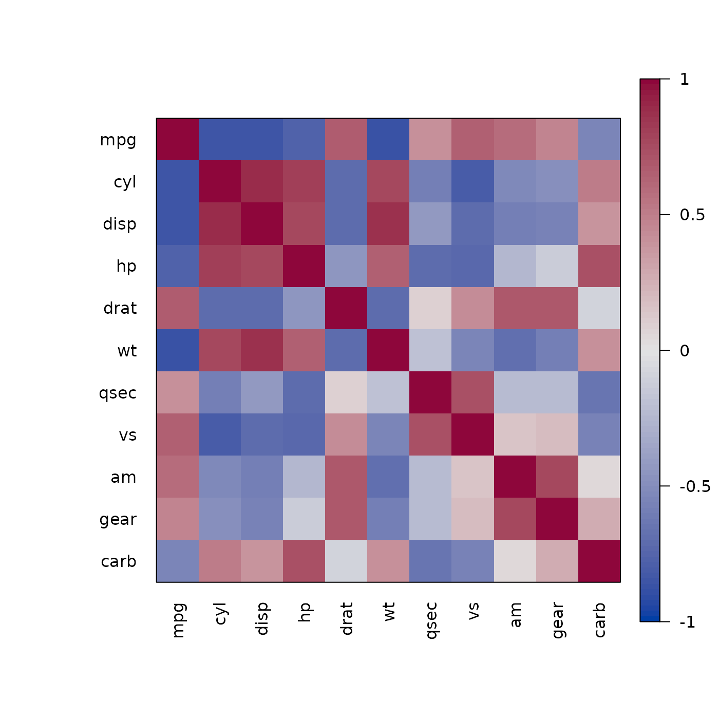
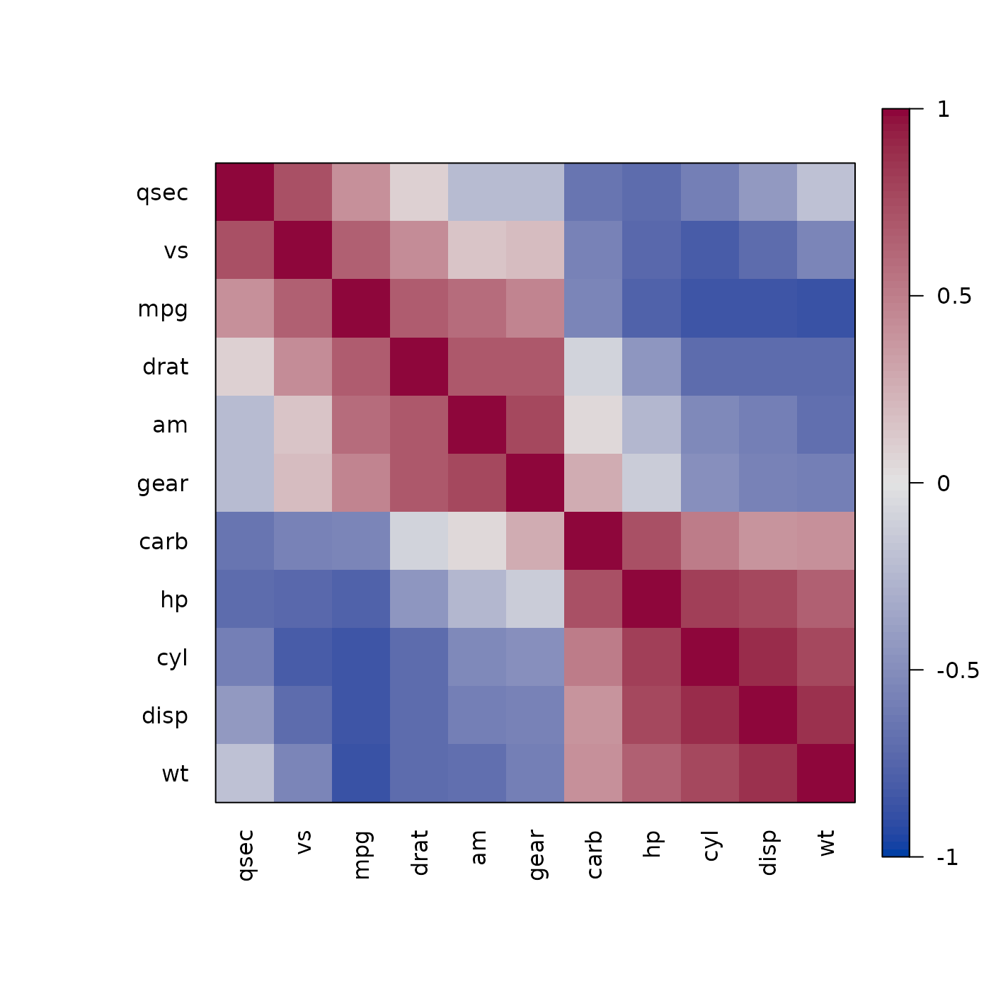
The reordering clearly shows that there are two groups of highly correlated variables and these two groups have a strong negative correlation with each other.
Visualization options
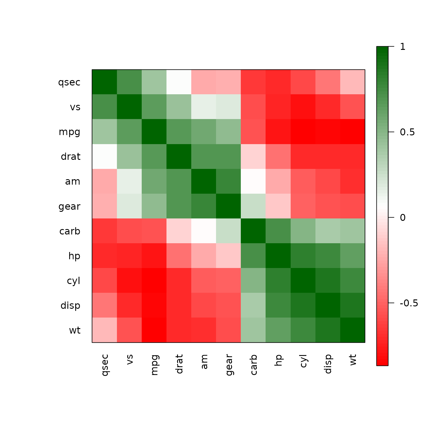
Here are some options. Many packages represent high correlations as blue and low correlations as red. We can set the colors that way or use other colors.
pimage(m, order = "AOE", col = rev(bluered()), diag = FALSE, upper_tri = FALSE)
pimage(m, order = "AOE", col = colorRampPalette(c("red", "white", "darkgreen"))(100))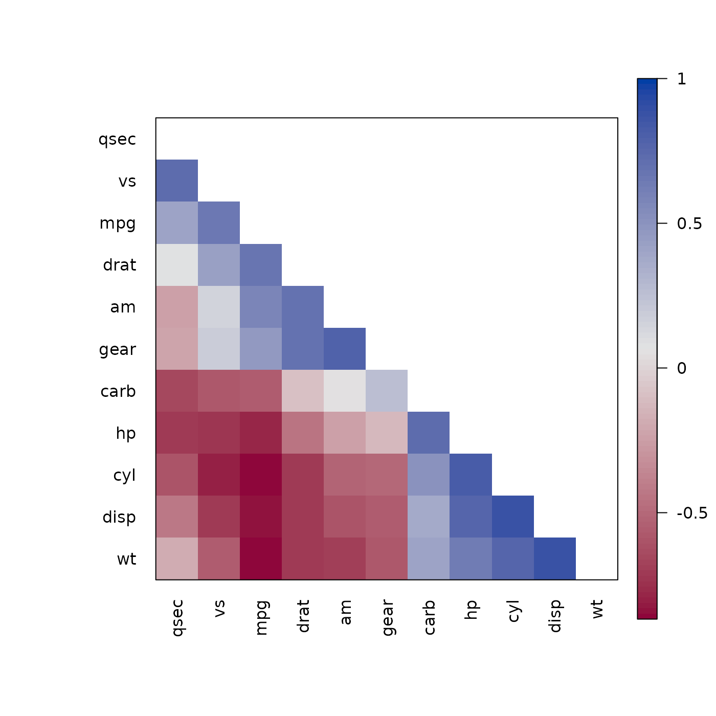
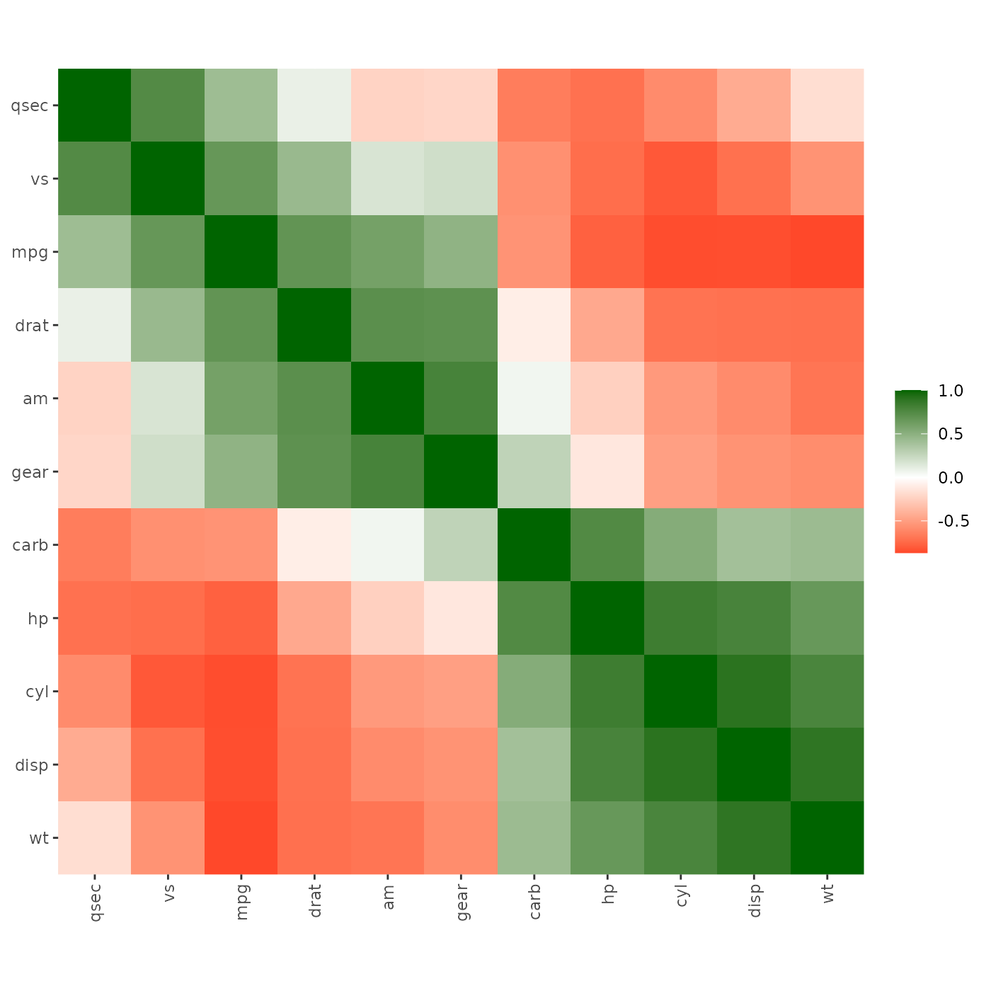
The plots are also available in ggplot2 versions.
library("ggplot2")

red_blue <- scale_fill_gradient2(
    low = scales::muted("red"),
    mid = "white",
    high = scales::muted("blue"),
    na.value = "white",
    midpoint = 0)

ggpimage(m, order = "AOE", diag = FALSE, upper_tri = FALSE) + red_blue
## Scale for fill is already present.
## Adding another scale for fill, which will replace the existing scale.
ggpimage(m, order = "AOE") + scale_fill_gradient2(low = "red", high = "darkgreen")## Scale for fill is already present.
## Adding another scale for fill, which will replace the existing scale.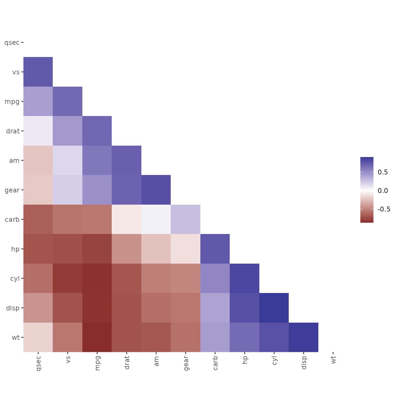
Using other seriation methods
We can apply any seriation method for distances to create an order. First, we convert the correlation matrix into a distance matrix using \(d_{ij} = \sqrt{1 - m_{ij}}\). Then we can use the distances for seriation and use the resulting order to rearrange the rows and columns of the correlation matrix.
d <- as.dist(sqrt(1 - m))

o <- seriate(d, "MDS")
pimage(m , order = c(o, o), main = "MDS", col = rev(bluered()))

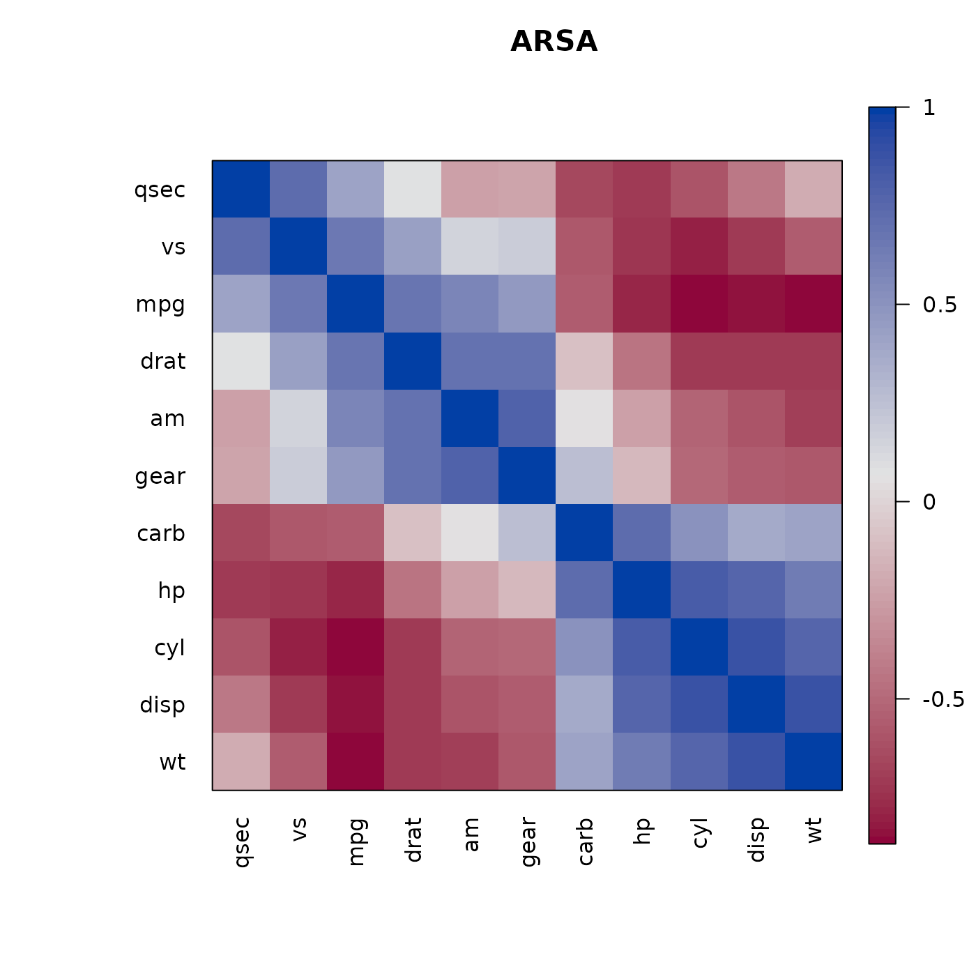
o <- seriate(d, "ARSA")
pimage(m , order = c(o, o), main = "ARSA", col = rev(bluered()))

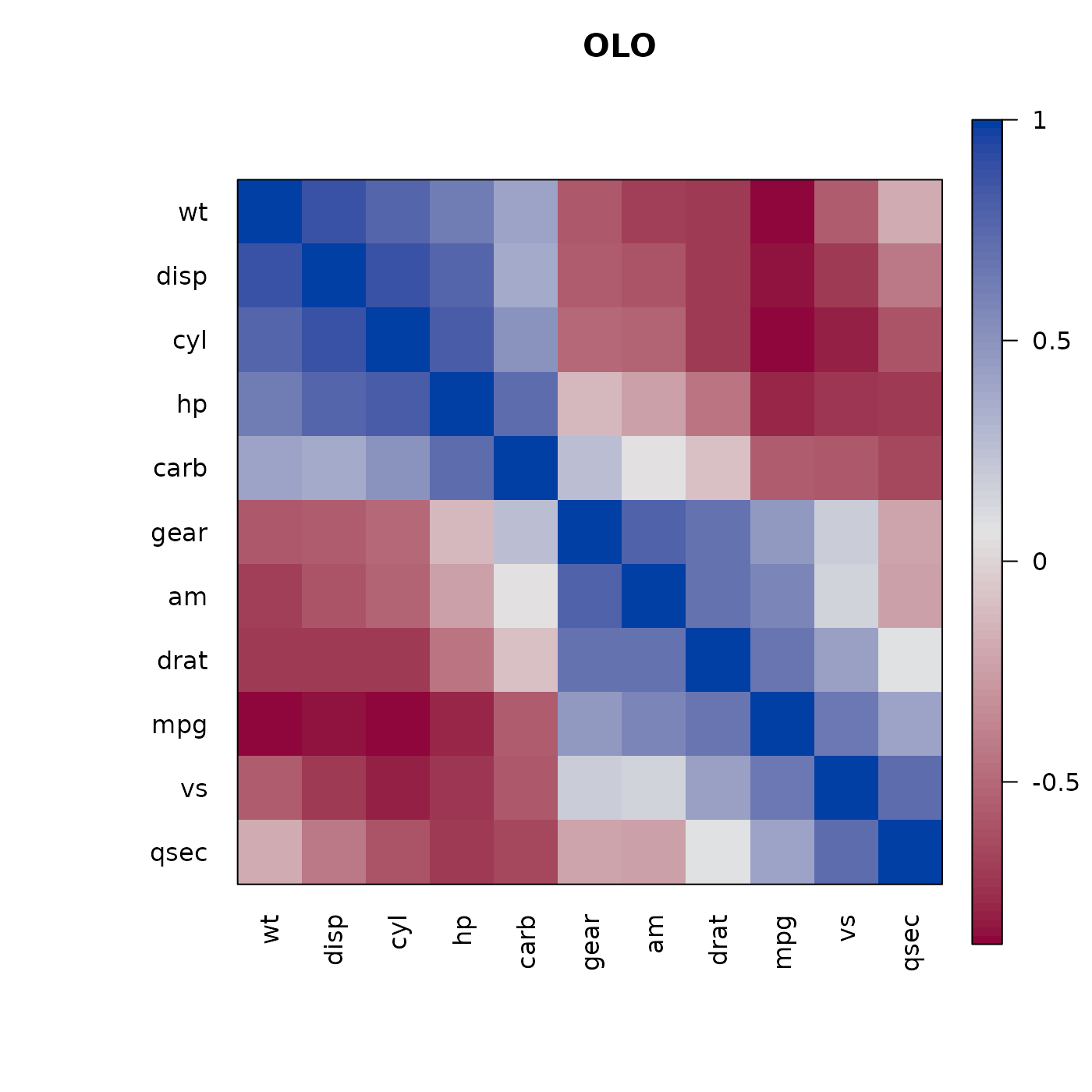
o <- seriate(d, "OLO")
pimage(m , order = c(o, o), main = "OLO", col = rev(bluered()))

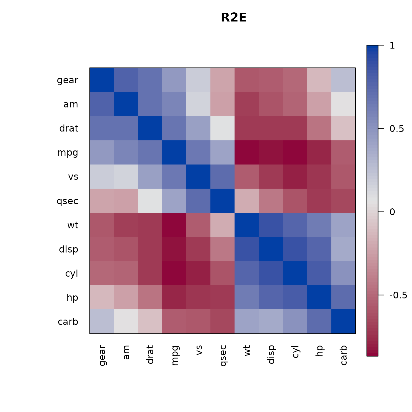
o <- seriate(d, "R2E")
pimage(m , order = c(o, o), main = "R2E", col = rev(bluered()))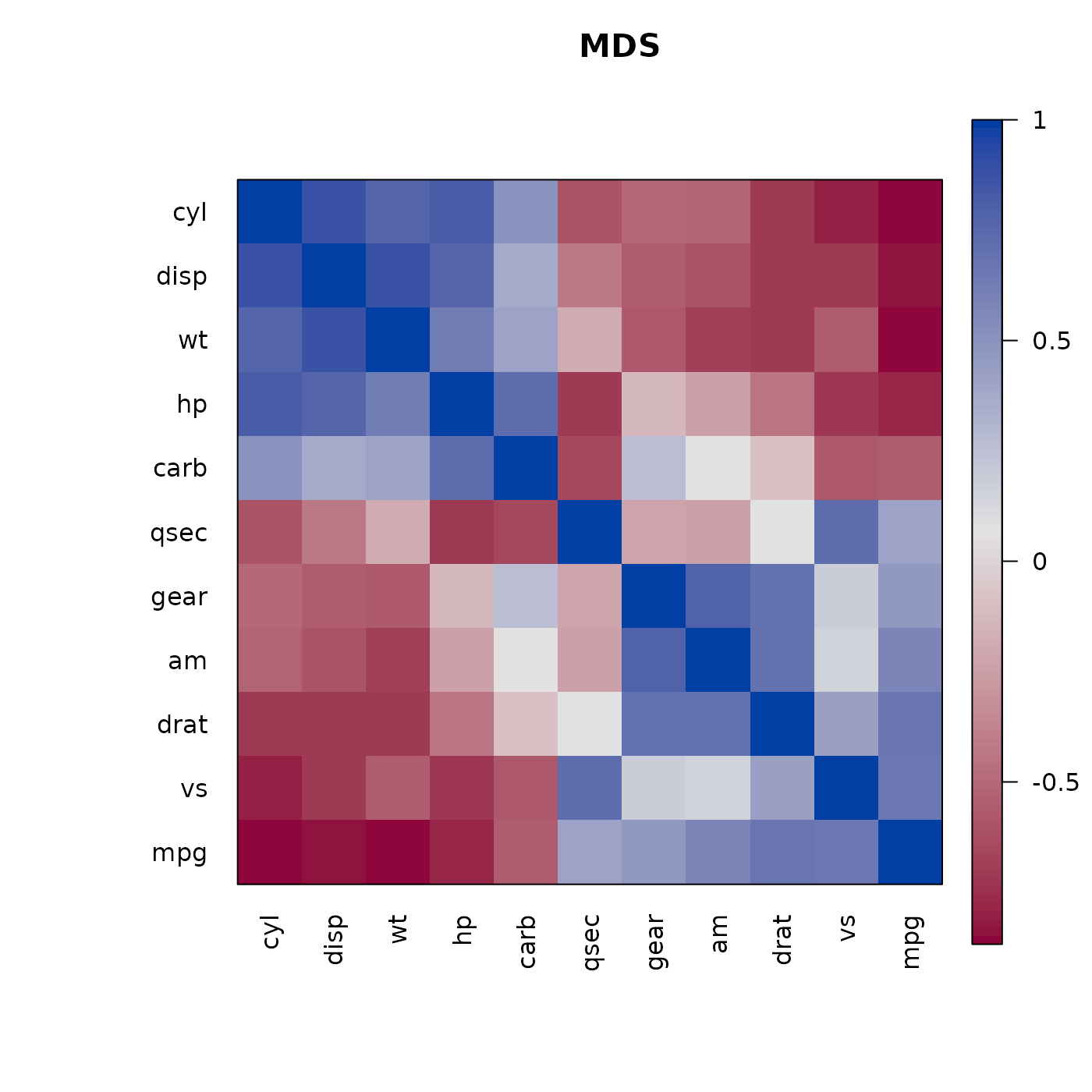
Other packages
Several other packages can be used to visualize and explore correlation structure. Some of these packages support reordering with the seriation package.
Package corrgram
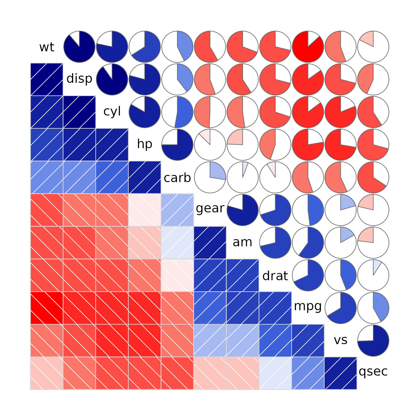
The order argument in corrgram accepts methods from package seriation.
if (!require("corrgram")) install.packages("corrgram")## Loading required package: corrgram
library("corrgram")

corrgram(m, order = "OLO")
corrgram(m, order = "OLO", lower.panel=panel.shade, upper.panel=panel.pie)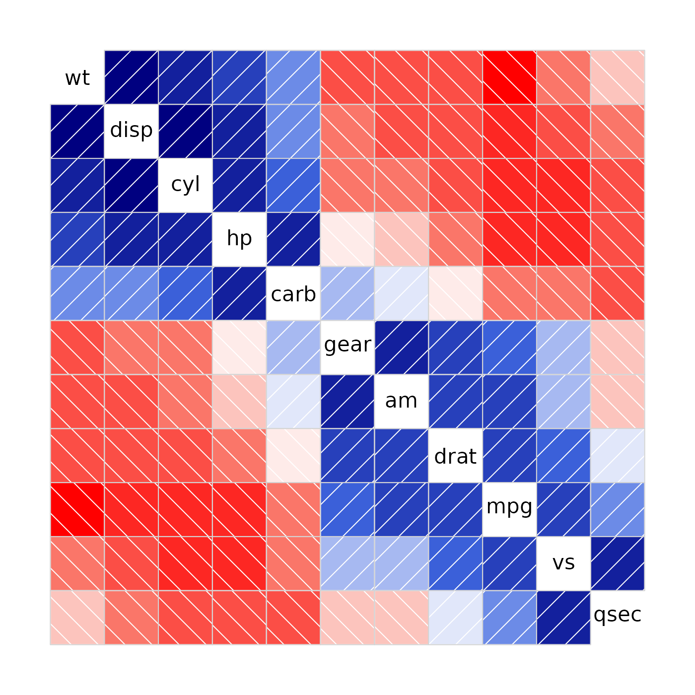
Package corrr
The function rearrange() in package corrr accepts some methods from
seriation. Here is a complete example that uses method
"R2E".
if (!require("corrr")) install.packages("corrr")## Loading required package: corrr
library("corrr")

x <- datasets::mtcars |>
       correlate() |>
       focus(-cyl, -vs, mirror = TRUE) |>  # remove 'cyl' and 'vs'
       rearrange(method = "R2E") |>
       shave()
## Correlation computed with
## • Method: 'pearson'
## • Missing treated using: 'pairwise.complete.obs'
rplot(x)## Warning: `aes_string()` was deprecated in ggplot2 3.0.0.
## ℹ Please use tidy evaluation idioms with `aes()`.
## ℹ See also `vignette("ggplot2-in-packages")` for more information.
## ℹ The deprecated feature was likely used in the corrr package.
## Please report the issue at <https://github.com/tidymodels/corrr/issues>.
## This warning is displayed once per session.
## Call `lifecycle::last_lifecycle_warnings()` to see where this warning was
## generated.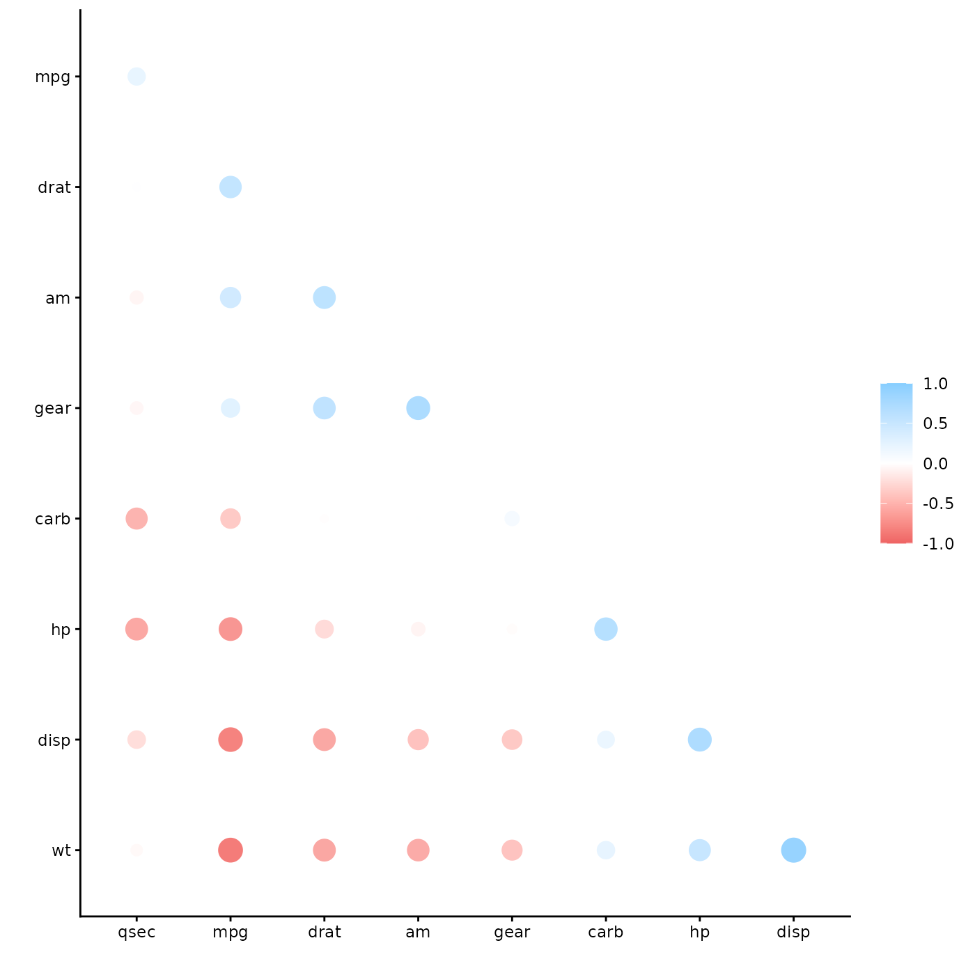
Package corrplot
Package corrplot
offers many visualization methods. Orders from package seriation can be
used by permuting the correlation matrix before it is passed to
corrplot().
if (!require("corrplot")) install.packages("corrplot")## Loading required package: corrplot## corrplot 0.95 loaded
library("corrplot")

d <- as.dist(sqrt(1 - m))
o <- seriate(d, "R2E")
m_R2E <- permute(m, c(o,o))

corrplot(m_R2E , order = "original")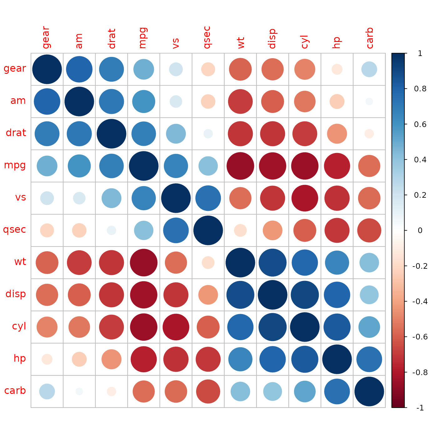
References
- Michael Hahsler, Kurt Hornik and Christian Buchta, Getting Things in Order: An Introduction to the R Package seriation, Journal of Statistical Software, 25(3), 2008. DOI: 10.18637/jss.v025.i03
- Friendly, M. (2002): Corrgrams: Exploratory Displays for Correlation Matrices. , (4), 316–324. DOI: 10.1198/000313002533