NBMiner: Mine NB-Frequent Itemsets or NB-Precise Rules

Mines NB-frequent itemsets or NB-precise rules.

Usage

NBMiner(data, parameter, control = NULL, ...)

Arguments

data: object of class arules::transactions.
parameter: an NBMinerParameter object or a named list of its parameters. Use NBMinerParameters() to estimate the model parameters.
control: an NBMinerControl object or a named list of control options. verbose and debug are logical options that control progress and diagnostic output.
...: named parameter overrides applied to parameter before mining. For example, use rules = TRUE to mine rules or change pi or theta.

Value

An object of class arules::itemsets or arules::rules, depending on the rules parameter. Estimated precision is stored in the quality slot.

Details

Mines NB-frequent itemsets or NB-precise rules (Hahsler, 2006) are non-spurious patterns that occur significantly more often in the data than one would expect if the items were independent. Under independence, we model each item's frequency as a Poisson count with an item specific rate, and models variation in those rates with a Gamma distribution. Mixing the Poisson counts over the Gamma rates gives a negative binomial distribution. This flexible baseline captures the skewed frequency distributions common in transaction data: a few items occur often, while many occur rarely. The model parameters for the independence model can be estimated from the data using NBMinerParameters().

NBMiner considers for an itemset adding each possible other item. Given the independent baseline it predicts how many extensions would reach each frequency by chance. The pi parameter sets the minimum predicted precision for accepting extensions. Here, precision means the predicted proportion of accepted extensions that are true associations under the model. Only extensions with a precision of at least pi are accepted.

The theta parameter controls pruning during search. For a larger itemset, it sets the required fraction of its immediate subsets that must support the itemset as an NB-frequent pattern. A value of 1 is most restrictive requiring all subsets also to be NB-frequent; 0 relaxes this condition. The intermediate default value 0.5 balances pruning with the chance of retaining associations whose items have different frequencies.

maxlen limits the longest itemset considered, and minlen can set a minimum length for returned patterns.

The mining algorithm uses a depth-first search implemented in Java.

Details can be found in Hahsler (2006).

References

Michael Hahsler. A model-based frequency constraint for mining associations from transaction data. Data Mining and Knowledge Discovery, 13(2):137-166, September 2006. doi:10.1007/s10618-005-0026-2

Examples

data("Agrawal")

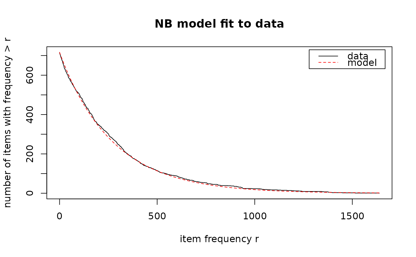
# Estimate independence model parameters
param <- NBMinerParameters(Agrawal.db, trim = 0)
#> using Expectation Maximization for missing zero class
#> iteration = 1 , zero class = 3 , k = 0.9862909 , m = 277.9777 
#> iteration = 2 , zero class = 3 , k = 0.9862909 , m = 277.9777 
#> total items =  719 
#> 
#> Goodness of fit/chi-square test on binned count data
#>   H0: Observed counts match the expected proportions.
#>   Bins:  10 
#>   X-squared =  5.778414  with  9  degrees of freedom
#>   p.value =  0.7618744 
#> 


# Mine non-spurious patterns
itemsets_NB <- NBMiner(Agrawal.db,
                       parameter = param,
                       pi = 0.99,
                       theta = 0.5,
                       minlen = 2L)

inspect(head(itemsets_NB))
#>     items                                precision
#> [1] {item217, item539}                   1.0000000
#> [2] {item222, item365, item478, item716} 1.0000000
#> [3] {item220, item452}                   1.0000000
#> [4] {item225, item299}                   0.9999951
#> [5] {item253, item438, item660, item849} 1.0000000
#> [6] {item214, item648}                   0.9993312

# Compare with the known patterns used to generate the data
num_correct <- function(itemsets, patterns)
    table(factor(rowSums(is.subset(itemsets, patterns)) > 0,
          c(FALSE, TRUE)))

# How many found itemsets are subsets of the patterns used in the db?
num_correct(itemsets_NB, Agrawal.pat)
#> 
#> FALSE  TRUE 
#>     0  2603 

# Compare with the same number of the most frequent itemsets
itemsets_supp <-  eclat(Agrawal.db, parameter = list(supp = 0.001, minlen = 2))
#> Eclat
#> 
#> parameter specification:
#>  tidLists support minlen maxlen            target  ext
#>     FALSE   0.001      2     10 frequent itemsets TRUE
#> 
#> algorithmic control:
#>  sparse sort verbose
#>       7   -2    TRUE
#> 
#> Absolute minimum support count: 20 
#> 
#> create itemset ... 
#> set transactions ...[716 item(s), 20000 transaction(s)] done [0.02s].
#> sorting and recoding items ... [656 item(s)] done [0.00s].
#> creating sparse bit matrix ... [656 row(s), 20000 column(s)] done [0.00s].
#> writing  ... [10217 set(s)] done [0.40s].
#> Creating S4 object  ... done [0.00s].
itemsets_supp <- head(sort(itemsets_supp, by = "support"), length(itemsets_NB))
num_correct(itemsets_supp, Agrawal.pat)
#> 
#> FALSE  TRUE 
#>   691  1912 

# we see that NBMiner is much more effective to recover the true patterns.


# Mine NB-precise rules
rules_NB <- NBMiner(Agrawal.db,
                    parameter = param,
                    pi = 0.99,
                    theta = 0.5,
                    rules = TRUE)
rules_NB
#> set of 5617 rules 

inspect(head(rules_NB))
#>     lhs                                    rhs       precision
#> [1] {item648}                           => {item548} 0.9982046
#> [2] {item1, item85}                     => {item520} 1.0000000
#> [3] {item508}                           => {item559} 1.0000000
#> [4] {item636, item648}                  => {item853} 1.0000000
#> [5] {item76, item669, item722, item879} => {item808} 1.0000000
#> [6] {item99, item823}                   => {item860} 1.0000000