Insert dummy cities into a distance matrix

Inserts dummy cities into a TSP problem. A dummy city has the same, constant distance (0) to all other cities and is infinitely far from other dummy cities. A dummy city can be used to transform a shortest Hamiltonian path problem (i.e., finding an optimal linear order) into a shortest Hamiltonian cycle problem which can be solved by a TSP solver (Garfinkel 1985).

Usage

insert_dummy(x, n = 1, const = 0, inf = Inf, label = "dummy")

# S3 method for class 'TSP'
insert_dummy(x, n = 1, const = 0, inf = Inf, label = "dummy")

# S3 method for class 'ATSP'
insert_dummy(x, n = 1, const = 0, inf = Inf, label = "dummy")

# S3 method for class 'ETSP'
insert_dummy(x, n = 1, const = 0, inf = Inf, label = "dummy")

Arguments

x: an object with a TSP problem.
n: number of dummy cities.
const: distance of the dummy cities to all other cities.
inf: distance between dummy cities.
label: labels for the dummy cities. If only one label is given, it is reused for all dummy cities.

Value

returns an object of the same class as x.

Details

Several dummy cities can be used together with a TSP solver to perform rearrangement clustering (Climer and Zhang 2006).

The dummy cities are inserted after the other cities in x.

A const of 0 is guaranteed to work if the TSP finds the optimal solution. For heuristics returning suboptimal solutions, a higher const (e.g., 2 * max(x)) might provide better results.

References

Sharlee Climer, Weixiong Zhang (2006): Rearrangement Clustering: Pitfalls, Remedies, and Applications, Journal of Machine Learning Research 7(Jun), pp. 919–943.

R.S. Garfinkel (1985): Motivation and modelling (chapter 2). In: E. L. Lawler, J. K. Lenstra, A.H.G. Rinnooy Kan, D. B. Shmoys (eds.) The traveling salesman problem - A guided tour of combinatorial optimization, Wiley & Sons.

Author

Michael Hahsler

Examples

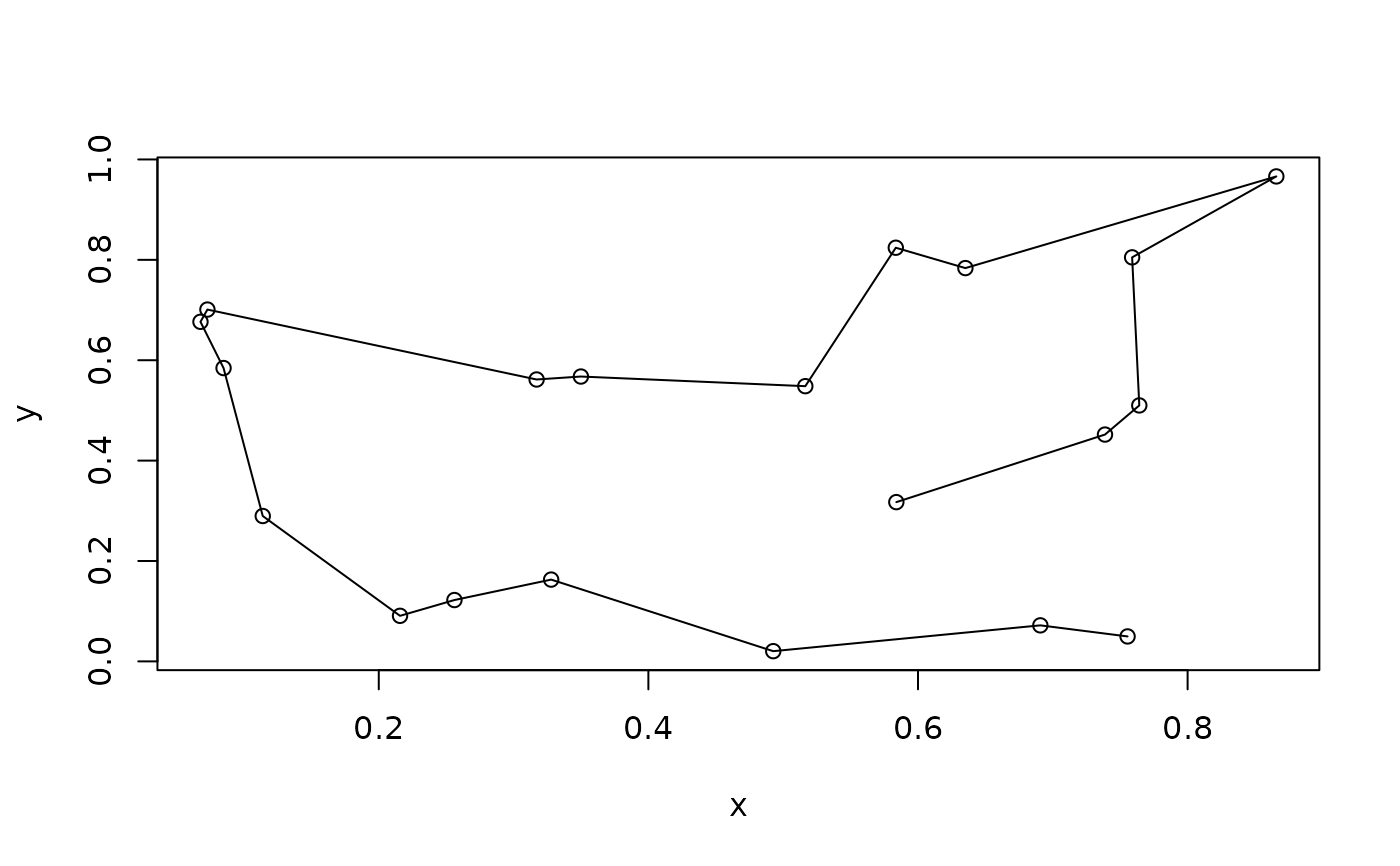
## Example 1: Find a short Hamiltonian path
set.seed(1000)
x <- data.frame(x = runif(20), y = runif(20), row.names = LETTERS[1:20])

tsp <- TSP(dist(x))

## add a dummy city to cut the tour into a path
tsp <- insert_dummy(tsp, label = "cut")
tour <- solve_TSP(tsp)
tour
#> object of class ‘TOUR’ 
#> result of method ‘arbitrary_insertion+two_opt’ for 21 cities
#> tour length: 3.145743 

plot(x)
lines(x[cut_tour(tour, cut = "cut"),])



## Example 2: Rearrangement clustering of the iris dataset
set.seed(1000)
data("iris")
tsp <- TSP(dist(iris[-5]))

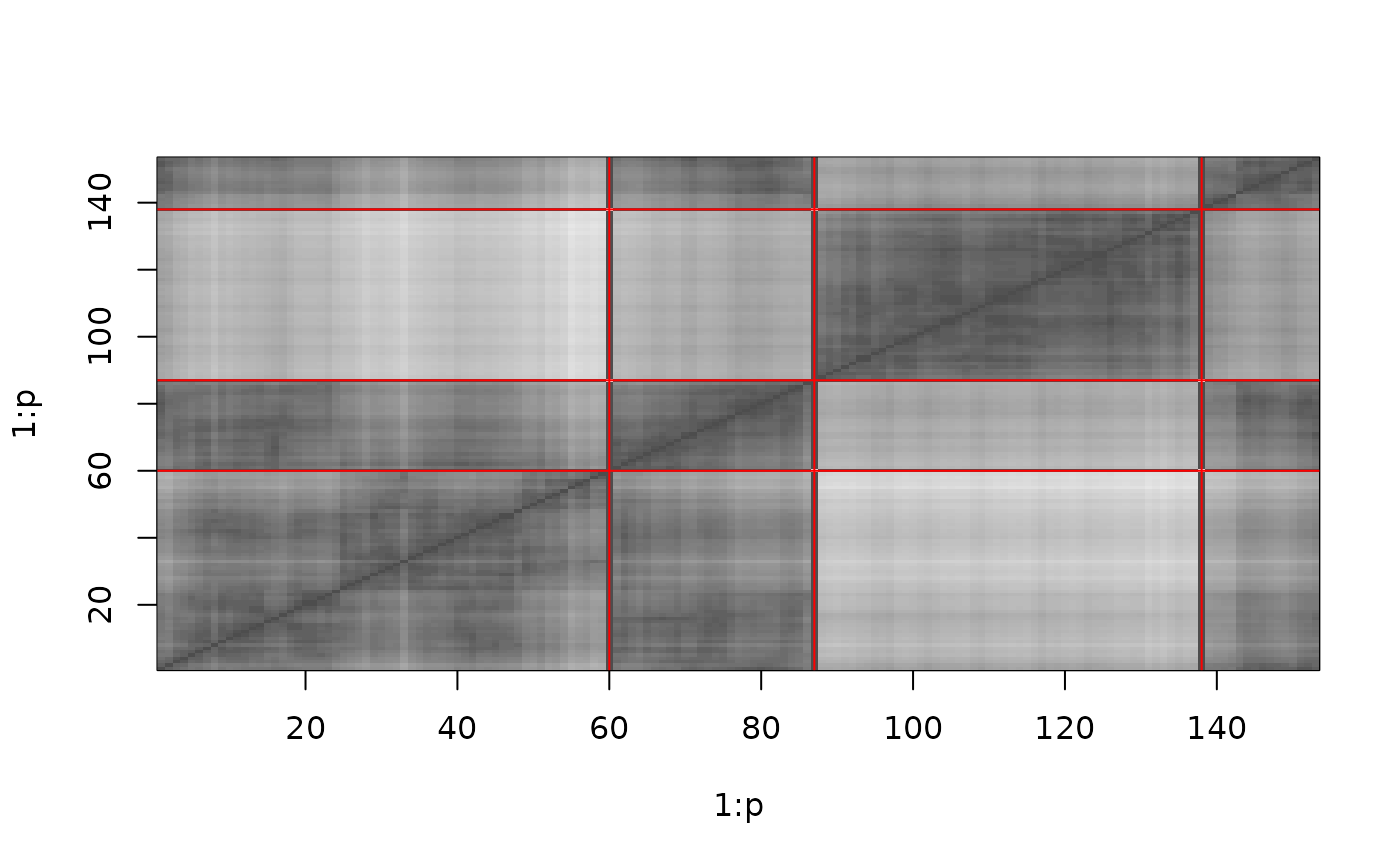
## insert 2 dummy cities to create 2 clusters
tsp_dummy <- insert_dummy(tsp, n = 3, label = "boundary")

## get a solution for the TSP
tour <- solve_TSP(tsp_dummy)

## plot the reordered distance matrix with the dummy cities as lines separating
## the clusters
image(tsp_dummy, tour)
abline(h = which(labels(tour)=="boundary"), col = "red")
abline(v = which(labels(tour)=="boundary"), col = "red")


## plot the original data with paths connecting the points in each cluster
plot(iris[,c(2,3)], col = iris[,5])
paths <- cut_tour(tour, cut = "boundary")
for(p in paths) lines(iris[p, c(2,3)])


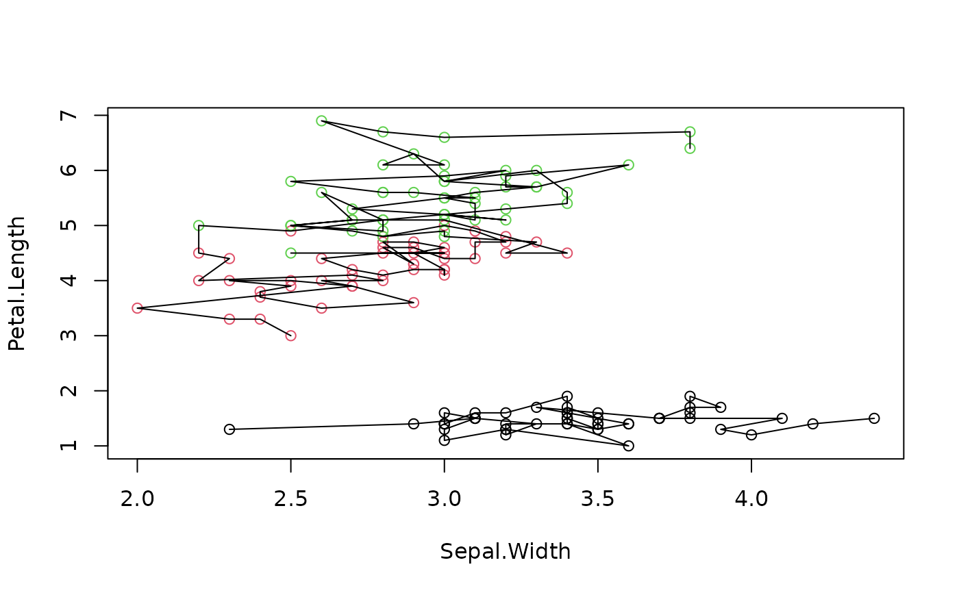## Note: The clustering is not perfect!