TSP solution methods
Michael Hahsler and Kurt Hornik
Source:vignettes/solution_methods.Rmd
solution_methods.RmdThis vignette uses the R package TSP (Hahsler and Hornik 2007). Please cite the
package and the accompanying Journal of Statistical Software paper (see
citation("TSP")) when you use it in your work.
Finding the shortest tour is NP-hard, so the number of tours that would have to be checked for an exact solution grows factorially with the number of cities. For this reason, TSP offers fast heuristics that find good (but not necessarily optimal) tours and an interface to the exact solver Concorde. This vignette describes the implemented methods and shows how to choose and compare them. All methods are called through the same function:
solve_TSP(x, method, control, ...)where x is a TSP, ATSP or
ETSP problem, method selects the algorithm,
and additional arguments (or the list control) set
method-specific parameters. The result is a TOUR object.
See ?solve_TSP for the complete list of parameters.
Overview of the methods
| Method argument | Algorithm | Type | Problems | Control parameters |
|---|---|---|---|---|
"identity", "random"
|
Order in the data / random order | construction | TSP, ATSP |
rep, opt,
verbose
|
"nn" |
Nearest neighbor | construction | TSP, ATSP |
start, rep, opt,
verbose
|
"repetitive_nn" |
Nearest neighbor from every start city | construction | TSP, ATSP |
opt, verbose
|
"nearest_insertion" |
Nearest insertion | construction | TSP, ATSP |
start, rep, opt,
verbose
|
"farthest_insertion" |
Farthest insertion | construction | TSP, ATSP |
start, rep, opt,
verbose
|
"cheapest_insertion" |
Cheapest insertion | construction | TSP, ATSP |
start, rep, opt,
verbose
|
"arbitrary_insertion" |
Arbitrary insertion | construction | TSP, ATSP |
start, rep, opt,
verbose
|
"two_opt" |
2-opt exchange | improvement | TSP, ATSP |
tour, two_opt_repetitions,
rep, opt, verbose
|
"or_opt" |
Or-opt segment insertion | improvement | TSP, ATSP |
tour, max_segment,
rep, opt, verbose
|
"three_opt" |
3-opt exchange | improvement | TSP, ATSP |
tour, rep, opt,
verbose
|
"sa" |
Simulated annealing | improvement | TSP, ATSP |
tour, local_move,
temp, tmax, maxit,
trace, rep, opt,
verbose
|
"concorde" |
Concorde (exact, branch-and-cut) | external solver | TSP, ETSP |
clo, precision,
keep_files, verbose, seed
|
"linkern" |
Chained Lin-Kernighan | external solver | TSP, ETSP |
clo, precision,
keep_files, verbose, seed
|
Most heuristics accept the following common control parameters:
-
rep: the number of random restarts. The best tour found is returned. -
opt: refine the constructed tour by local search:"two"(2-opt),"or"(Or-opt),"three"(3-opt), or"two+or"(2-opt and Or-opt alternately). The oldertwo_opt = TRUEis deprecated; useopt = "two". -
start: the first city for nearest neighbor and insertion algorithms. -
verbose: show progress and the parameters that are used.
If no method is given, solve_TSP() uses arbitrary
insertion followed by 2-opt improvement. Construction heuristics build a
tour from scratch, while improvement heuristics start with an existing
tour (given as tour) and try to shorten it. If no tour is
supplied to an improvement heuristic, a random tour is used.
Tour construction heuristics
These algorithms create a tour from scratch.
Nearest neighbor
The nearest neighbor algorithm (Rosenkrantz et
al. 1977) is a simple greedy procedure. It starts with a randomly
chosen city (or the city given by start) and repeatedly
appends the nearest city that has not been visited yet. It is very fast,
but typically has to make long “jumps” at the end of the tour to reach
the remaining cities.
The repetitive variant ("repetitive_nn") runs the
algorithm once from every city and returns the shortest tour found.
Insertion algorithms
All insertion algorithms (Rosenkrantz et al. 1977) start with a tour consisting of a single city and repeatedly insert a city \(k\) that is not yet on the tour between two consecutive tour cities \(i\) and \(j\) so that the increase in tour length
\[d(i,k) + d(k,j) - d(i,j)\]
is minimal. They differ in how the city to be inserted is chosen:
- Nearest insertion chooses the city closest to any city on the tour.
- Farthest insertion chooses the city farthest from the tour. This first establishes an outline of the whole tour and fills in details later. In practice, farthest insertion often produces better tours than the other insertion variants.
- Cheapest insertion chooses the city with the lowest insertion cost.
- Arbitrary insertion chooses a random city. It is the fastest variant.
For distances that obey the triangle inequality, nearest and cheapest insertion are related to Prim’s minimum spanning tree algorithm (Prim 1957) and guarantee tours that are at most twice the optimal length.
Tour improvement heuristics
These heuristics modify existing tours to improve them. If no starting tour is specified then typically a random tour is used as the starting point.
2-opt is very effective. Many methods have for convenience the
control parameter opt which automatically applies a
refinement to the constructed tour. It can be "two"
(2-opt), "or" (Or-opt), "three" (3-opt), or
"two+or" (2-opt and Or-opt alternately until neither
improves the tour). For example,
solve_TSP(x, method = "nn", opt = "two+or"). Without a
method, solve_TSP() uses arbitrary insertion with
opt = "two". The older control parameter
two_opt = TRUE is deprecated.
2-opt
Two-opt (Croes 1958) repeatedly removes
two edges from the tour and reconnects the two resulting paths in the
only other possible way (which is equivalent to reversing a part of the
tour) whenever this shortens the tour. The procedure stops at a
2-optimal tour, i.e., a local optimum for this neighborhood.
"two_opt_repetitions" can be used to restart the algorithm
from random tours.
Or-opt
Or-opt (Or 1976) moves a segment of 1
to max_segment consecutive cities (default 3) to a
different position in the tour, whenever this shortens the tour. For
symmetric problems, the segment may also be inserted in reverse order.
Or-opt can relocate a misplaced city or a small group of cities in a
single step, which 2-opt cannot do, while 2-opt removes crossing edges,
which Or-opt cannot do. The two methods complement each other, which is
why opt = "two+or" alternates between them. Or-opt only
needs a few moves to be checked and is about as fast as 2-opt.
3-opt
Three-opt (Bock 1958; Lin 1965) removes three edges, which splits the tour into three parts, and reconnects them in the best of all possible ways (including reversing parts). Its neighborhood contains all 2-opt and Or-opt moves, so a 3-optimal tour is also 2-optimal and Or-optimal. The price is a run time of \(O(n^3)\) for each pass over all triples of edges, which makes 3-opt practical only for small to medium problems (up to a few thousand cities). For asymmetric problems, only the reconnection that does not reverse any part of the tour is used.
Simulated annealing
Simulated annealing (Kirkpatrick et al.
1983) uses random local moves (reversal of a random sub-tour) and
accepts moves that make the tour longer with a probability that
decreases as the temperature is lowered. This allows the search to
escape local optima. The implementation uses stats::optim()
with method "SANN". The method is usually much slower than
2-opt and needs tuning of the cooling schedule (temp,
tmax, maxit). By default, only 10,000
evaluations are used to keep the run time short, so a larger
maxit is needed for competitive results.
Improving an existing tour
Improvement heuristics can be applied to any tour, including a tour that was created outside of TSP. For example, we can refine a nearest neighbor tour with 2-opt, Or-opt, and 3-opt, and then use a long simulated annealing run for further improvement.
library(TSP)
data(USCA50)
set.seed(1234)

nn <- solve_TSP(USCA50, method = "nn", start = 1)
opt2 <- solve_TSP(USCA50, method = "two_opt", tour = nn)
optor <- solve_TSP(USCA50, method = "or_opt", tour = opt2)
opt3 <- solve_TSP(USCA50, method = "three_opt", tour = optor)
sa <- solve_TSP(USCA50, method = "sa", tour = opt3, maxit = 50000)

c(nn = tour_length(nn), two_opt = tour_length(opt2),
  or_opt = tour_length(optor), three_opt = tour_length(opt3),
  sa = tour_length(sa))
#>        nn   two_opt    or_opt three_opt        sa
#>     17203     16324     15499     14497     14497
We see how improvement methods reduce the tour length. The same
refinements can be requested directly when a tour is constructed using
opt. We set the same random number seed inside the loop to
get the same nearest-neighbor tour. We run each algorithm with 10 random
restarts.
opts <- c("none", "two", "or", "two+or", "three")
## nearest neighbor breaks ties randomly. We reset the seed so every
## refinement starts from the same nearest neighbor tour.
len <- sapply(opts, function(o) {
  set.seed(1234)
  tour <- solve_TSP(USCA50, method = "nn", rep = 10,
    opt = if (o == "none") NULL else o)
  tour_length(tour)
})
#> Warning: executing %dopar% sequentially: no parallel backend registered
len
#>   none    two     or two+or  three
#>  15208  14826  14497  14510  14497

## the optimal tour length (found by Concorde) is 14497
barplot(len / 14497 * 100 - 100, xlab = "opt",
  ylab = "percent excess over optimum in %")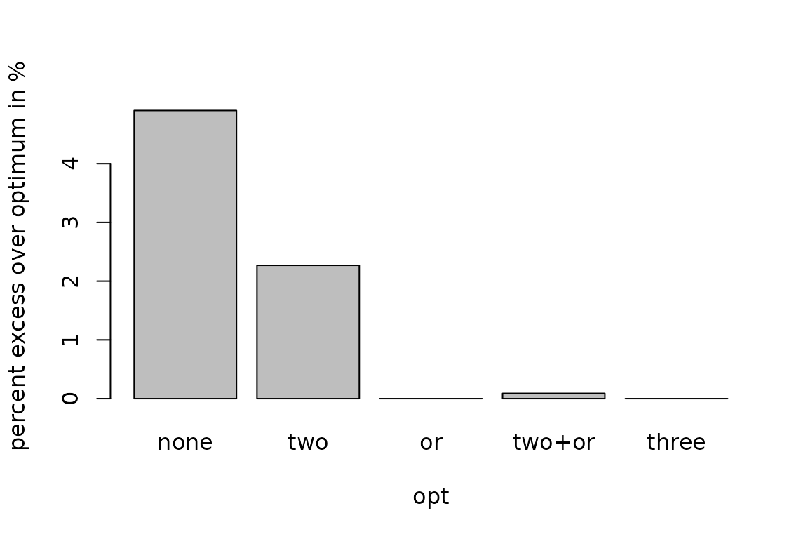
State-of-the-art solvers
Concorde (Applegate et al. 2006) is
currently one of the best exact solvers for symmetric TSPs. It uses the
branch-and-cut method (Padberg and Rinaldi
1990) which iteratively tightens a linear programming relaxation
of the problem. The Chained Lin-Kernighan heuristic (Applegate et al. 2003), an extension of the
Lin-Kernighan heuristic (Lin and Kernighan
1973), is a very fast heuristic that finds excellent tours for
large instances. Both are accessed via the "concorde" and
"linkern" methods, but require that the Concorde
executables are installed separately. See
vignette("concorde") for details.
Asymmetric and Euclidean problems
All heuristics above work with asymmetric problems
(ATSP). Solvers that only handle symmetric problems use an
automatic reformulation as a symmetric TSP with twice as many cities
(see ?reformulate_ATSP_as_TSP).
Euclidean problems (ETSP) are converted into distance
matrices for the built-in heuristics, which needs memory proportional to
the square of the number of cities. Only "concorde" and
"linkern" work with ETSP objects directly.
Reproducibility
Many methods are randomized (e.g., "random",
"nn" with a random start,
"arbitrary_insertion", "sa", and all methods
with rep > 1). They use R’s global random-number stream.
Calling set.seed() before solve_TSP() makes a
run reproducible, and every call advances the stream as any other R
function that draws random numbers does.
Parallel execution
Repetitions (including "repetitive_nn") are run using
the foreach package and can be executed in parallel by
registering a backend before calling solve_TSP().
library(doParallel)
#> Loading required package: foreach
#> Loading required package: iterators
#> Loading required package: parallel
registerDoParallel()
solve_TSP(USCA50, rep = 100)
#> object of class 'TOUR'
#> result of method 'arbitrary_insertion+two_opt_rep_100' for 50 cities
#> tour length: 14497
For parallel repetitions, one random number per repetition is drawn
from R’s global stream in the main R process and used to seed the
iteration (on the main process or a worker). The results are therefore
reproducible with set.seed() independent of the backend and
the number of workers.