 R package dbscan - Density-Based Spatial Clustering of Applications with Noise (DBSCAN) and Related Algorithms



Introduction
This R package (Hahsler et al. 2019) provides a fast C++ (re)implementation of several density-based algorithms with a focus on the DBSCAN family for clustering spatial data. The package includes:
Clustering
-
DBSCAN: Density-based spatial clustering of applications with noise (Ester et al. 1996).
-
FOSC: Framework for optimal selection of clusters for unsupervised and semisupervised clustering of hierarchical cluster trees (Campello et al. 2013).
-
HDBSCAN: Hierarchical DBSCAN with simplified hierarchy extraction (Campello et al. 2015).
-
Jarvis-Patrick Clustering: Clustering using a similarity measure based on shared near neighbors (Jarvis and Patrick 1973).
-
OPTICS/OPTICSXi: Ordering points to identify the clustering structure and cluster extraction methods
-
SNN Clustering: Shared nearest neighbor clustering (Ertöz et al. 2003).
Outlier Detection
- LOF: Local outlier factor algorithm (Breunig et al. 2000).
- GLOSH: Global-Local Outlier Score from Hierarchies algorithm (Campello et al. 2015).
Cluster Evaluation
- DBCV: Density-based clustering validation (Moulavi et al. 2014).
Fast Nearest-Neighbor Search (using kd-trees)
- kNN search
- Fixed-radius NN search
The implementations use the kd-tree data structure (from library ANN)
for faster k-nearest neighbor search, and are for Euclidean distance
typically faster than the native R implementations (e.g., dbscan in
package fpc), or the implementations in
WEKA,
ELKI and Python’s
scikit-learn.
The following R packages use dbscan:
AnimalSequences,
autoFlagR,
bioregion,
clayringsmiletus,
CLONETv2,
clusterWebApp,
cordillera,
CPC,
crosshap,
cyclicwave,
daltoolbox,
DataSimilarity,
diceR,
discoCVI,
dobin,
doc2vec,
dPCP,
DrData,
EHRtemporalVariability,
emcAdr,
eventstream,
evprof,
fastml,
FCPS,
fdacluster,
flowcluster,
flownet,
FuelDeep3D,
funtimes,
HaploVar,
immunaut,
karyotapR,
ksharp,
LLMing,
LOMAR,
maotai,
MapperAlgo,
mditools,
metaCluster,
metasnf,
mlr3cluster,
neuroim2,
oclust,
omicsTools,
openSkies,
opticskxi,
OTclust,
outlierensembles,
outlierMBC,
pagoda2,
parameters,
performance,
pguIMP,
phynotype,
PiC,
quickOutlier,
rarefun,
rcrisp,
Rhobots,
riemannianStats,
riskutility,
rMultiNet,
rtemis,
SampleCore,
seriation,
sfdep,
sfnetworks,
sharp,
smotefamily,
snap,
spCF,
spdep,
specmine,
spNetwork,
squat,
ssel,
ssMRCD,
STATassist,
stdbscan,
stream,
SuperCell,
synr,
tbnb,
TextAnalysisR,
tidyclust,
tidylearn,
tidySEM,
tlsR,
VBphenoR,
VIProDesign,
weird
To cite package ‘dbscan’ in publications use:
Hahsler M, Piekenbrock M, Doran D (2019). “dbscan: Fast Density-Based Clustering with R.” Journal of Statistical Software, 91(1), 1-30. <doi:10.18637/jss.v091.i01> https://doi.org/10.18637/jss.v091.i01.
@Article{,
  title = {dbscan: Fast Density-Based Clustering with {R}},
  author = {Michael Hahsler and Matthew Piekenbrock and Derek Doran},
  journal = {Journal of Statistical Software},
  year = {2019},
  volume = {91},
  number = {1},
  pages = {1--30},
  doi = {10.18637/jss.v091.i01},
}
Installation
Stable CRAN version: Install from within R with
install.packages("dbscan")
Current development version: Install from r-universe.
install.packages("dbscan",
    repos = c("https://mhahsler.r-universe.dev",
              "https://cloud.r-project.org/"))
Usage
Load the package and use the numeric variables in the iris dataset
library("dbscan")

data("iris")
x <- as.matrix(iris[, 1:4])
DBSCAN
db <- dbscan(x, eps = .42, minPts = 5)
db
## DBSCAN clustering for 150 objects.
## Parameters: eps = 0.42, minPts = 5
## Using euclidean distances and borderpoints = TRUE
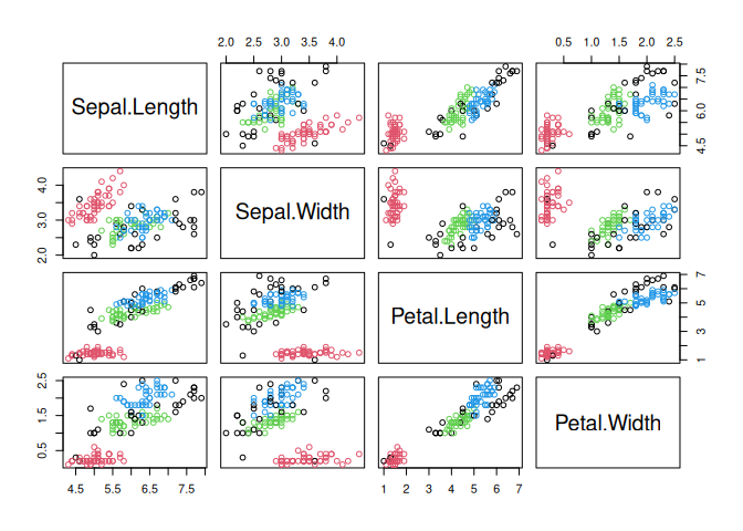
## The clustering contains 3 cluster(s) and 29 noise points.
##
##  0  1  2  3
## 29 48 37 36
##
## Available fields: cluster, eps, minPts, metric, borderPoints
Visualize the resulting clustering (noise points are shown in black).
pairs(x, col = db$cluster + 1L)
OPTICS
opt <- optics(x, eps = 1, minPts = 4)
opt
## OPTICS ordering/clustering for 150 objects.
## Parameters: minPts = 4, eps = 1, eps_cl = NA, xi = NA
## Available fields: order, reachdist, coredist, predecessor, minPts, eps,
##                   eps_cl, xi
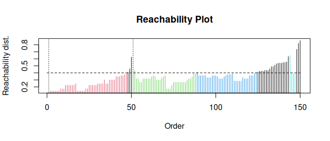
Extract DBSCAN-like clustering from OPTICS and create a reachability plot (extracted DBSCAN clusters at eps_cl=.4 are colored)
opt <- extractDBSCAN(opt, eps_cl = .4)
plot(opt)
HDBSCAN
hdb <- hdbscan(x, minPts = 4)
hdb
## HDBSCAN clustering for 150 objects.
## Parameters: minPts = 4
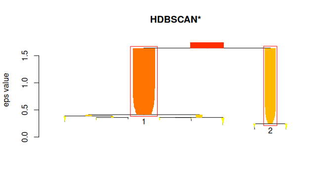
## The clustering contains 2 cluster(s) and 0 noise points.
##
##   1   2
## 100  50
##
## Available fields: cluster, minPts, coredist, cluster_scores,
##                   membership_prob, outlier_scores, hc
Visualize the hierarchical clustering as a simplified tree. HDBSCAN finds 2 stable clusters.
plot(hdb, show_flat = TRUE)
Using dbscan with tidyverse
dbscan provides for all clustering algorithms tidy(), augment(),
and glance() so they can be easily used with tidyverse, ggplot2 and
tidymodels.
library(tidyverse)
db <- x %>% dbscan(eps = .42, minPts = 5)
Get cluster statistics as a tibble
tidy(db)
## # A tibble: 4 × 3
##   cluster  size noise
##   <fct>   <int> <lgl>
## 1 0          29 TRUE
## 2 1          48 FALSE
## 3 2          37 FALSE
## 4 3          36 FALSE
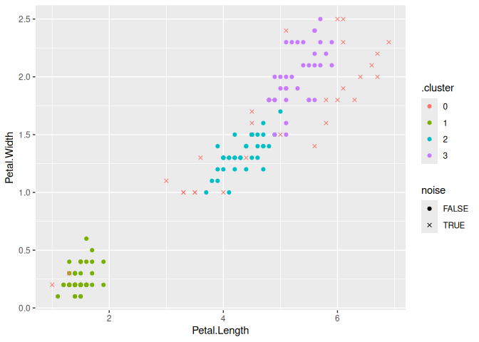
Visualize the clustering with ggplot2 (use an x for noise points)
augment(db, x) %>%
  ggplot(aes(x = Petal.Length, y = Petal.Width)) +
    geom_point(aes(color = .cluster, shape = noise)) +
    scale_shape_manual(values=c(19, 4))
Using dbscan from Python
R, the R package dbscan, and the Python package rpy2 need to be
installed.
import pandas as pd
import numpy as np

### prepare data
iris = pd.read_csv('https://archive.ics.uci.edu/ml/machine-learning-databases/iris/iris.data',
                   header = None,
                   names = ['SepalLength', 'SepalWidth', 'PetalLength', 'PetalWidth', 'Species'])
iris_numeric = iris[['SepalLength', 'SepalWidth', 'PetalLength', 'PetalWidth']]

# get R dbscan package
from rpy2.robjects import packages
dbscan = packages.importr('dbscan')

# enable automatic conversion of pandas dataframes to R dataframes
from rpy2.robjects import pandas2ri
pandas2ri.activate()

db = dbscan.dbscan(iris_numeric, eps = 0.5, MinPts = 5)
print(db)
## DBSCAN clustering for 150 objects.
## Parameters: eps = 0.5, minPts = 5
## Using euclidean distances and borderpoints = TRUE
## The clustering contains 2 cluster(s) and 17 noise points.
##
##  0  1  2
## 17 49 84
##
## Available fields: cluster, eps, minPts, dist, borderPoints
# get the cluster assignment vector
labels = np.array(db.rx('cluster'))
labels
## array([[1, 1, 1, 1, 1, 1, 1, 1, 1, 1, 1, 1, 1, 1, 1, 1, 1, 1, 1, 1, 1, 1,
##         1, 1, 1, 1, 1, 1, 1, 1, 1, 1, 1, 1, 1, 1, 1, 1, 1, 1, 1, 0, 1, 1,
##         1, 1, 1, 1, 1, 1, 2, 2, 2, 2, 2, 2, 2, 0, 2, 2, 0, 2, 2, 2, 2, 2,
##         2, 2, 0, 2, 2, 2, 2, 2, 2, 2, 2, 2, 2, 2, 2, 2, 2, 2, 2, 2, 2, 0,
##         2, 2, 2, 2, 2, 0, 2, 2, 2, 2, 0, 2, 2, 2, 2, 2, 2, 0, 0, 2, 0, 0,
##         2, 2, 2, 2, 2, 2, 2, 0, 0, 2, 2, 2, 0, 2, 2, 2, 2, 2, 2, 2, 2, 0,
##         2, 2, 0, 0, 2, 2, 2, 2, 2, 2, 2, 2, 2, 2, 2, 2, 2, 2]],
##       dtype=int32)
License
The dbscan package is licensed under the GNU General Public License (GPL) Version 3. The OPTICSXi R implementation was directly ported from the ELKI framework’s Java implementation (GNU AGPLv3), with permission by the original author, Erich Schubert.
Changes
- List of changes from NEWS.md