Convert a Continuous Variable into a Categorical Variable

This function implements several basic unsupervised methods to convert a continuous variable into a categorical variable (factor) using different binning strategies. For convenience, a whole data.frame can be discretized (i.e., all numeric columns are discretized).

Usage

discretize(
  x,
  method = "frequency",
  breaks = 3,
  labels = NULL,
  include.lowest = TRUE,
  right = FALSE,
  dig.lab = 3,
  ordered_result = FALSE,
  infinity = FALSE,
  onlycuts = FALSE,
  categories = NULL,
  ...
)

discretizeDF(df, methods = NULL, default = NULL)

Arguments

x: a numeric vector (continuous variable).
method: discretization method. Available are: "interval" (equal interval width), "frequency" (equal frequency), "cluster" (k-means clustering) and "fixed" (categories specifies interval boundaries). Note that equal frequency does not achieve perfect equally sized groups if the data contains duplicated values.
breaks, categories: either number of categories or a vector with boundaries for discretization (all values outside the boundaries will be set to NA). categories is deprecated, use breaks instead.
labels: character vector; labels for the levels of the resulting category. By default, labels are constructed using "(a,b]" interval notation. If labels = FALSE, simple integer codes are returned instead of a factor..
include.lowest: logical; should the first interval be closed to the left?
right: logical; should the intervals be closed on the right (and open on the left) or vice versa?
dig.lab: integer; number of digits used to create labels.
ordered_result: logical; return a ordered factor?
infinity: logical; should the first/last break boundary changed to +/-Inf?
onlycuts: logical; return only computed interval boundaries?
...: for method "cluster" further arguments are passed on to kmeans.
df: data.frame; each numeric column in the data.frame is discretized.
methods: named list of lists or a data.frame; the named list contains lists of discretization parameters (see parameters of discretize()) for each numeric column (see details). If no discretization is specified for a column, then the default settings for discretize() are used. Note: the names have to match exactly. If a data.frame is specified, then the discretization breaks in this data.frame are applied to df.
default: named list; parameters for discretize() used for all columns not specified in methods.

Value

discretize() returns a factor representing the categorized continuous variable with attribute "discretized:breaks" indicating the used breaks or and "discretized:method" giving the used method. If onlycuts = TRUE is used, a vector with the calculated interval boundaries is returned.

discretizeDF() returns a discretized data.frame.

Details

Discretize calculates breaks between intervals using various methods and then uses base::cut() to convert the numeric values into intervals represented as a factor.

Discretization may fail for several reasons. Some reasons are

A variable contains only a single value. In this case, the variable should be dropped or directly converted into a factor with a single level (see factor).
Some calculated breaks are not unique. This can happen for method frequency with very skewed data (e.g., a large portion of the values is 0). In this case, non-unique breaks are dropped with a warning. It would be probably better to look at the histogram of the data and decide on breaks for the method fixed.

discretize only implements unsupervised discretization. See arulesCBA::discretizeDF.supervised() in package arulesCBA for supervised discretization.

discretizeDF() applies discretization to each numeric column. Individual discretization parameters can be specified in the form: methods = list(column_name1 = list(method = ,...), column_name2 = list(...)). If no discretization method is specified for a column, then the discretization in default is applied (NULL invokes the default method in discretize()). The special method "none" can be specified to suppress discretization for a column.

Author

Michael Hahsler

Examples

data(iris)
x <- iris[, 1]

### look at the distribution before discretizing
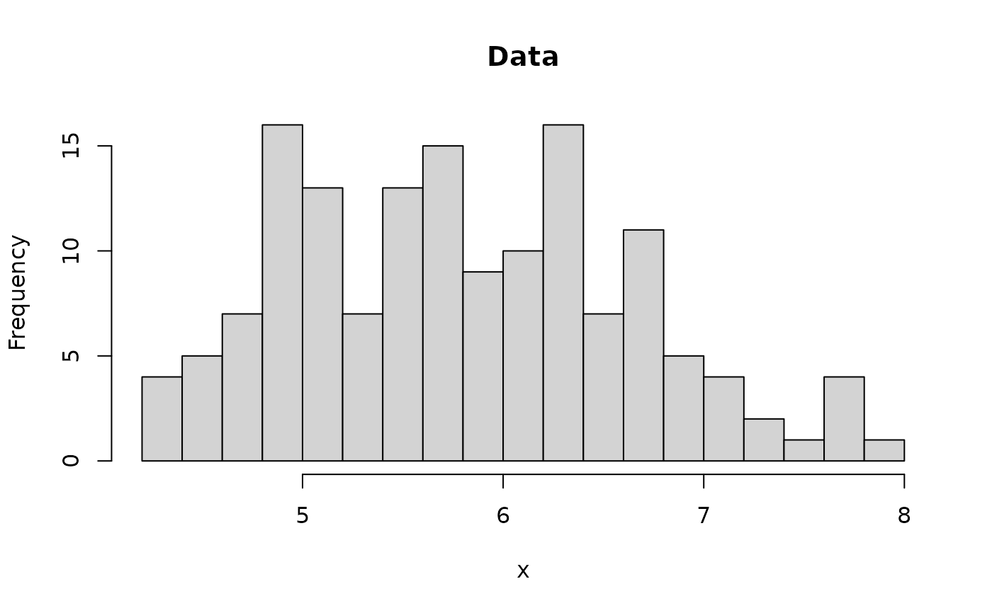
hist(x, breaks = 20, main = "Data")


def.par <- par(no.readonly = TRUE) # save default
layout(mat = rbind(1:2, 3:4))

### convert continuous variables into categories (there are 3 types of flowers)
### the default method is equal frequency
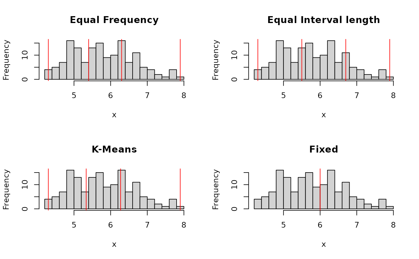
table(discretize(x, breaks = 3))
#> 
#> [4.3,5.4) [5.4,6.3) [6.3,7.9] 
#>        46        53        51 
hist(x, breaks = 20, main = "Equal Frequency")
abline(v = discretize(x,
  breaks = 3,
  onlycuts = TRUE
), col = "red")
# Note: the frequencies are not exactly equal because of ties in the data

### equal interval width
table(discretize(x, method = "interval", breaks = 3))
#> 
#> [4.3,5.5) [5.5,6.7) [6.7,7.9] 
#>        52        70        28 
hist(x, breaks = 20, main = "Equal Interval length")
abline(v = discretize(x,
  method = "interval", breaks = 3,
  onlycuts = TRUE
), col = "red")

### k-means clustering
table(discretize(x, method = "cluster", breaks = 3))
#> 
#>  [4.3,5.33) [5.33,6.27)  [6.27,7.9] 
#>          46          53          51 
hist(x, breaks = 20, main = "K-Means")
abline(v = discretize(x,
  method = "cluster", breaks = 3,
  onlycuts = TRUE
), col = "red")

### user-specified (with labels)
table(discretize(x,
  method = "fixed", breaks = c(-Inf, 6, Inf),
  labels = c("small", "large")
))
#> 
#> small large 
#>    83    67 
hist(x, breaks = 20, main = "Fixed")
abline(v = discretize(x,
  method = "fixed", breaks = c(-Inf, 6, Inf),
  onlycuts = TRUE
), col = "red")


par(def.par) # reset to default

### prepare the iris data set for association rule mining
### use default discretization
irisDisc <- discretizeDF(iris)
head(irisDisc)
#>   Sepal.Length Sepal.Width Petal.Length Petal.Width Species
#> 1    [4.3,5.4)   [3.2,4.4]     [1,2.63) [0.1,0.867)  setosa
#> 2    [4.3,5.4)   [2.9,3.2)     [1,2.63) [0.1,0.867)  setosa
#> 3    [4.3,5.4)   [3.2,4.4]     [1,2.63) [0.1,0.867)  setosa
#> 4    [4.3,5.4)   [2.9,3.2)     [1,2.63) [0.1,0.867)  setosa
#> 5    [4.3,5.4)   [3.2,4.4]     [1,2.63) [0.1,0.867)  setosa
#> 6    [5.4,6.3)   [3.2,4.4]     [1,2.63) [0.1,0.867)  setosa

### discretize all numeric columns differently
irisDisc <- discretizeDF(iris, default = list(
  method = "interval", breaks = 2,
  labels = c("small", "large")
))
head(irisDisc)
#>   Sepal.Length Sepal.Width Petal.Length Petal.Width Species
#> 1        small       large        small       small  setosa
#> 2        small       small        small       small  setosa
#> 3        small       large        small       small  setosa
#> 4        small       small        small       small  setosa
#> 5        small       large        small       small  setosa
#> 6        small       large        small       small  setosa

### specify discretization for the petal columns and don't discretize the others
irisDisc <- discretizeDF(iris,
  methods = list(
    Petal.Length = list(
      method = "frequency", breaks = 3,
      labels = c("short", "medium", "long")
    ),
    Petal.Width = list(
      method = "frequency", breaks = 2,
      labels = c("narrow", "wide")
    )
  ),
  default = list(method = "none")
)
head(irisDisc)
#>   Sepal.Length Sepal.Width Petal.Length Petal.Width Species
#> 1          5.1         3.5        short      narrow  setosa
#> 2          4.9         3.0        short      narrow  setosa
#> 3          4.7         3.2        short      narrow  setosa
#> 4          4.6         3.1        short      narrow  setosa
#> 5          5.0         3.6        short      narrow  setosa
#> 6          5.4         3.9        short      narrow  setosa

### discretize new data using the same discretization scheme as the
###   data.frame supplied in methods. Note: NAs may occure if a new
###   value falls outside the range of values observed in the
###   originally discretized table (use argument infinity = TRUE in
###   discretize to prevent this case.)
discretizeDF(iris[sample(1:nrow(iris), 5), ], methods = irisDisc)
#>     Sepal.Length Sepal.Width Petal.Length Petal.Width    Species
#> 69           6.2         2.2       medium        wide versicolor
#> 49           5.3         3.7        short      narrow     setosa
#> 25           4.8         3.4        short      narrow     setosa
#> 39           4.4         3.0        short      narrow     setosa
#> 117          6.5         3.0         long        wide  virginica