 This work is licensed under the
Creative Commons Attribution 4.0 International License. For questions please contact
Michael Hahsler.
This work is licensed under the
Creative Commons Attribution 4.0 International License. For questions please contact
Michael Hahsler.Additional material for the course “Introduction to Data Mining”
This work is licensed under the
Creative Commons Attribution 4.0 International License. For questions please contact
Michael Hahsler.
Linear regression models the value of a dependent variable $y$ (also called response) as as linear function of independent variabels $X_1, X_2, …, X_p$ (also called regressors, predictors, exogenous variables or covariates). Given $n$ observations the model is: \(y_i = \beta_0 + \beta_1 x_{i1} + \dots + \beta_p x_{ip} + \epsilon_i\)
where $\beta_0$ is the intercept, $\beta$ is a $p$-dimensional parameter vector learned from the data, and $\epsilon$ is the error term (called residuals).
Linear regression makes several assumptions:
set.seed(2000)
Load and shuffle data (flowers are in order by species)
data(iris)
x <- iris[sample(1:nrow(iris)),]
plot(x, col=x$Species)
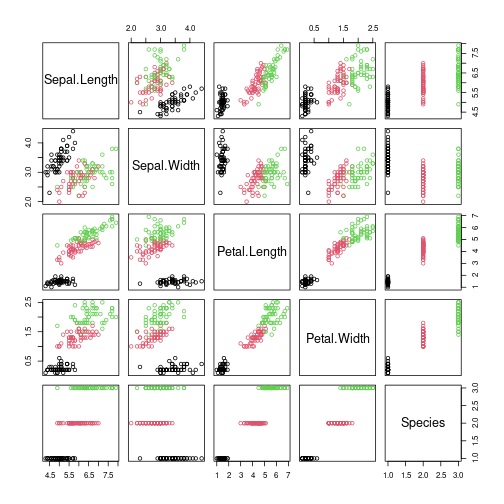
Make the data a little messy and add a useless feature
x[,1] <- x[,1] + rnorm(nrow(x))
x[,2] <- x[,2] + rnorm(nrow(x))
x[,3] <- x[,3] + rnorm(nrow(x))
x <- cbind(x[,-5], useless = mean(x[,1]) + rnorm(nrow(x)), Species = x[,5])

plot(x, col=x$Species)

summary(x)
##   Sepal.Length    Sepal.Width      Petal.Length      Petal.Width       useless            Species
##  Min.   :2.678   Min.   :0.6107   Min.   :-0.7134   Min.   :0.100   Min.   :2.923   setosa    :50
##  1st Qu.:5.048   1st Qu.:2.3062   1st Qu.: 1.8761   1st Qu.:0.300   1st Qu.:5.227   versicolor:50
##  Median :5.919   Median :3.1708   Median : 4.1017   Median :1.300   Median :5.905   virginica :50
##  Mean   :5.847   Mean   :3.1284   Mean   : 3.7809   Mean   :1.199   Mean   :5.884
##  3rd Qu.:6.696   3rd Qu.:3.9453   3rd Qu.: 5.5462   3rd Qu.:1.800   3rd Qu.:6.565
##  Max.   :8.810   Max.   :5.9747   Max.   : 7.7078   Max.   :2.500   Max.   :8.108
head(x)
##     Sepal.Length Sepal.Width Petal.Length Petal.Width  useless    Species
## 85      2.980229    1.463570     5.227091         1.5 5.711515 versicolor
## 104     5.096036    3.043735     5.186573         1.8 6.568673  virginica
## 30      4.361172    2.831668     1.860620         0.2 4.299253     setosa
## 53      8.125130    2.405599     5.526070         1.5 6.123879 versicolor
## 143     6.371932    1.565055     6.147013         1.9 6.552573  virginica
## 142     6.525973    3.696871     5.708392         2.3 5.221676  virginica
Create some training and learning data
train <- x[1:100,]
test <- x[101:150,]
Can we predict Petal.Width using the other variables?
lm uses a formula interface see ?lm for description
model1 <- lm(Petal.Width ~ Sepal.Length
            + Sepal.Width + Petal.Length + useless,
            data = train)
model1
##
## Call:
## lm(formula = Petal.Width ~ Sepal.Length + Sepal.Width + Petal.Length +
##     useless, data = train)
##
## Coefficients:
##  (Intercept)  Sepal.Length   Sepal.Width  Petal.Length       useless
##    -0.205886      0.019568      0.034062      0.308139      0.003917
coef(model1)
##  (Intercept) Sepal.Length  Sepal.Width Petal.Length      useless
## -0.205886022  0.019568449  0.034061702  0.308138700  0.003916688
Summary shows:
summary(model1)
##
## Call:
## lm(formula = Petal.Width ~ Sepal.Length + Sepal.Width + Petal.Length +
##     useless, data = train)
##
## Residuals:
##     Min      1Q  Median      3Q     Max
## -1.0495 -0.2033  0.0074  0.2038  0.8564
##
## Coefficients:
##               Estimate Std. Error t value Pr(>|t|)
## (Intercept)  -0.205886   0.287229  -0.717    0.475
## Sepal.Length  0.019568   0.032654   0.599    0.550
## Sepal.Width   0.034062   0.035493   0.960    0.340
## Petal.Length  0.308139   0.018185  16.944   <2e-16 ***
## useless       0.003917   0.035579   0.110    0.913
## ---
## Signif. codes:  0 '***' 0.001 '**' 0.01 '*' 0.05 '.' 0.1 ' ' 1
##
## Residual standard error: 0.3665 on 95 degrees of freedom
## Multiple R-squared:  0.7784,	Adjusted R-squared:  0.769
## F-statistic: 83.41 on 4 and 95 DF,  p-value: < 2.2e-16
Plotting the model produces diagnostic plots (see ? plot.lm). For example
to check for homoscedasticity (residual vs predicted value scatter plot should not look like a funnel)
and if the residuals are approximately normally distributed (Q-Q plot should be close to the straight line).
plot(model1, which = 1:2)


We try simpler models
model2 <- lm(Petal.Width ~ Sepal.Length + Sepal.Width + Petal.Length,
             data = train)
summary(model2)
##
## Call:
## lm(formula = Petal.Width ~ Sepal.Length + Sepal.Width + Petal.Length,
##     data = train)
##
## Residuals:
##     Min      1Q  Median      3Q     Max
## -1.0440 -0.2024  0.0099  0.1998  0.8513
##
## Coefficients:
##              Estimate Std. Error t value Pr(>|t|)
## (Intercept)  -0.18415    0.20757  -0.887    0.377
## Sepal.Length  0.01993    0.03232   0.617    0.539
## Sepal.Width   0.03392    0.03529   0.961    0.339
## Petal.Length  0.30800    0.01805  17.068   <2e-16 ***
## ---
## Signif. codes:  0 '***' 0.001 '**' 0.01 '*' 0.05 '.' 0.1 ' ' 1
##
## Residual standard error: 0.3646 on 96 degrees of freedom
## Multiple R-squared:  0.7783,	Adjusted R-squared:  0.7714
## F-statistic: 112.4 on 3 and 96 DF,  p-value: < 2.2e-16
No intercept
model3 <- lm(Petal.Width ~ Sepal.Length + Sepal.Width + Petal.Length - 1,
             data = train)
summary(model3)
##
## Call:
## lm(formula = Petal.Width ~ Sepal.Length + Sepal.Width + Petal.Length -
##     1, data = train)
##
## Residuals:
##      Min       1Q   Median       3Q      Max
## -1.03103 -0.19610 -0.00512  0.22643  0.82459
##
## Coefficients:
##               Estimate Std. Error t value Pr(>|t|)
## Sepal.Length -0.001684   0.021215  -0.079    0.937
## Sepal.Width   0.018595   0.030734   0.605    0.547
## Petal.Length  0.306659   0.017963  17.072   <2e-16 ***
## ---
## Signif. codes:  0 '***' 0.001 '**' 0.01 '*' 0.05 '.' 0.1 ' ' 1
##
## Residual standard error: 0.3642 on 97 degrees of freedom
## Multiple R-squared:  0.9376,	Adjusted R-squared:  0.9357
## F-statistic: 485.8 on 3 and 97 DF,  p-value: < 2.2e-16
Very simple model
model4 <- lm(Petal.Width ~ Petal.Length -1,
             data = train)
summary(model4)
##
## Call:
## lm(formula = Petal.Width ~ Petal.Length - 1, data = train)
##
## Residuals:
##      Min       1Q   Median       3Q      Max
## -0.97745 -0.19569  0.00779  0.25362  0.84550
##
## Coefficients:
##              Estimate Std. Error t value Pr(>|t|)
## Petal.Length 0.315864   0.008224   38.41   <2e-16 ***
## ---
## Signif. codes:  0 '***' 0.001 '**' 0.01 '*' 0.05 '.' 0.1 ' ' 1
##
## Residual standard error: 0.3619 on 99 degrees of freedom
## Multiple R-squared:  0.9371,	Adjusted R-squared:  0.9365
## F-statistic:  1475 on 1 and 99 DF,  p-value: < 2.2e-16
Compare models (Null hypothesis: all treatments=models have the same effect). Note: This only works for nested models. Models are nested only if one model contains all the predictors of the other model.
anova(model1, model2, model3, model4)
## Analysis of Variance Table
##
## Model 1: Petal.Width ~ Sepal.Length + Sepal.Width + Petal.Length + useless
## Model 2: Petal.Width ~ Sepal.Length + Sepal.Width + Petal.Length
## Model 3: Petal.Width ~ Sepal.Length + Sepal.Width + Petal.Length - 1
## Model 4: Petal.Width ~ Petal.Length - 1
##   Res.Df    RSS Df Sum of Sq      F Pr(>F)
## 1     95 12.761
## 2     96 12.762 -1 -0.001628 0.0121 0.9126
## 3     97 12.867 -1 -0.104641 0.7790 0.3797
## 4     99 12.968 -2 -0.101046 0.3761 0.6875
Models 1 is not significantly better than model 2. Model 2 is not significantly better than model 3. Model 3 is not significantly better than model 4! Use model 4 (simplest model)
Automatically looks for the smallest AIC (Akaike information criterion)
s1 <- step(lm(Petal.Width ~ . -Species, data=train))
## Start:  AIC=-195.88
## Petal.Width ~ (Sepal.Length + Sepal.Width + Petal.Length + useless +
##     Species) - Species
##
##                Df Sum of Sq    RSS      AIC
## - useless       1     0.002 12.762 -197.869
## - Sepal.Length  1     0.048 12.809 -197.504
## - Sepal.Width   1     0.124 12.884 -196.917
## <none>                      12.760 -195.882
## - Petal.Length  1    38.565 51.325  -58.699
##
## Step:  AIC=-197.87
## Petal.Width ~ Sepal.Length + Sepal.Width + Petal.Length
##
##                Df Sum of Sq    RSS     AIC
## - Sepal.Length  1     0.051 12.813 -199.47
## - Sepal.Width   1     0.123 12.885 -198.91
## <none>                      12.762 -197.87
## - Petal.Length  1    38.727 51.489  -60.38
##
## Step:  AIC=-199.47
## Petal.Width ~ Sepal.Width + Petal.Length
##
##                Df Sum of Sq    RSS     AIC
## - Sepal.Width   1     0.136 12.949 -200.41
## <none>                      12.813 -199.47
## - Petal.Length  1    44.727 57.540  -51.27
##
## Step:  AIC=-200.41
## Petal.Width ~ Petal.Length
##
##                Df Sum of Sq    RSS     AIC
## <none>                      12.949 -200.41
## - Petal.Length  1    44.625 57.574  -53.21
summary(s1)
##
## Call:
## lm(formula = Petal.Width ~ Petal.Length, data = train)
##
## Residuals:
##     Min      1Q  Median      3Q     Max
## -0.9848 -0.1873  0.0048  0.2466  0.8343
##
## Coefficients:
##              Estimate Std. Error t value Pr(>|t|)
## (Intercept)   0.02802    0.07431   0.377    0.707
## Petal.Length  0.31031    0.01689  18.377   <2e-16 ***
## ---
## Signif. codes:  0 '***' 0.001 '**' 0.01 '*' 0.05 '.' 0.1 ' ' 1
##
## Residual standard error: 0.3635 on 98 degrees of freedom
## Multiple R-squared:  0.7751,	Adjusted R-squared:  0.7728
## F-statistic: 337.7 on 1 and 98 DF,  p-value: < 2.2e-16
What if two variables are only important together? Interaction terms
are modeled with : or * in the formula (they are literally multiplied).
See ? formula.
model5 <- step(lm(Petal.Width ~ Sepal.Length * Sepal.Width * Petal.Length,
             data = train))
## Start:  AIC=-196.4
## Petal.Width ~ Sepal.Length * Sepal.Width * Petal.Length
##
##                                         Df Sum of Sq    RSS     AIC
## <none>                                               11.955 -196.40
## - Sepal.Length:Sepal.Width:Petal.Length  1   0.26511 12.220 -196.21
summary(model5)
##
## Call:
## lm(formula = Petal.Width ~ Sepal.Length * Sepal.Width * Petal.Length,
##     data = train)
##
## Residuals:
##      Min       1Q   Median       3Q      Max
## -1.10639 -0.18818  0.02376  0.17669  0.85773
##
## Coefficients:
##                                       Estimate Std. Error t value Pr(>|t|)
## (Intercept)                           -2.42072    1.33575  -1.812   0.0732 .
## Sepal.Length                           0.44836    0.23130   1.938   0.0556 .
## Sepal.Width                            0.59832    0.38446   1.556   0.1231
## Petal.Length                           0.72748    0.28635   2.541   0.0127 *
## Sepal.Length:Sepal.Width              -0.11151    0.06705  -1.663   0.0997 .
## Sepal.Length:Petal.Length             -0.08330    0.04774  -1.745   0.0843 .
## Sepal.Width:Petal.Length              -0.09407    0.08504  -1.106   0.2715
## Sepal.Length:Sepal.Width:Petal.Length  0.02010    0.01407   1.428   0.1566
## ---
## Signif. codes:  0 '***' 0.001 '**' 0.01 '*' 0.05 '.' 0.1 ' ' 1
##
## Residual standard error: 0.3605 on 92 degrees of freedom
## Multiple R-squared:  0.7924,	Adjusted R-squared:  0.7766
## F-statistic: 50.15 on 7 and 92 DF,  p-value: < 2.2e-16
anova(model5, model4)
## Analysis of Variance Table
##
## Model 1: Petal.Width ~ Sepal.Length * Sepal.Width * Petal.Length
## Model 2: Petal.Width ~ Petal.Length - 1
##   Res.Df    RSS Df Sum of Sq      F Pr(>F)
## 1     92 11.955
## 2     99 12.968 -7   -1.0129 1.1135 0.3614
Model 5 is not significantly better than model 4
test[1:5,]
##     Sepal.Length Sepal.Width Petal.Length Petal.Width  useless    Species
## 128     8.016904    1.541029     3.515360         1.8 6.110446  virginica
## 92      5.267566    4.064301     6.064320         1.4 4.937890 versicolor
## 50      5.461307    4.160921     1.117372         0.2 6.372570     setosa
## 134     6.055488    2.951358     4.598716         1.5 5.595099  virginica
## 8       4.899848    5.095657     1.085505         0.2 7.270446     setosa
test[1:5,]$Petal.Width
## [1] 1.8 1.4 0.2 1.5 0.2
predict(model4, test[1:5,])
##       128        92        50       134         8
## 1.1103744 1.9154981 0.3529372 1.4525672 0.3428715
Calculate the root-mean-square error (RMSE): less is better
RMSE <- function(predicted, true) mean((predicted-true)^2)^.5
RMSE(predict(model4, test), test$Petal.Width)
## [1] 0.3873689
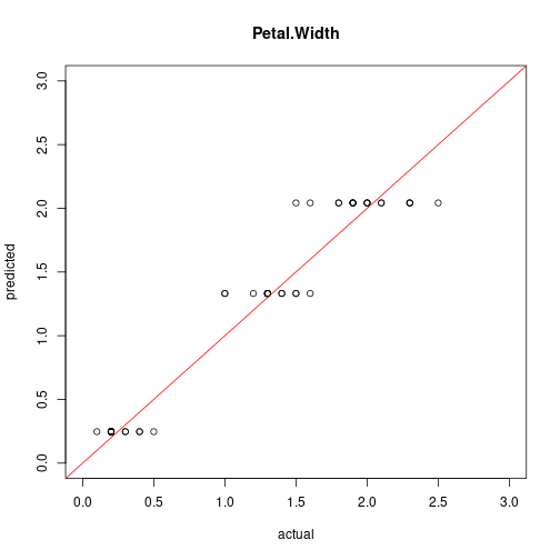
Compare predicted vs. actual values
plot(test[,"Petal.Width"], predict(model4, test),
  xlim=c(0,3), ylim=c(0,3), xlab = "actual", ylab = "predicted",
  main = "Petal.Width")
abline(0,1, col="red")
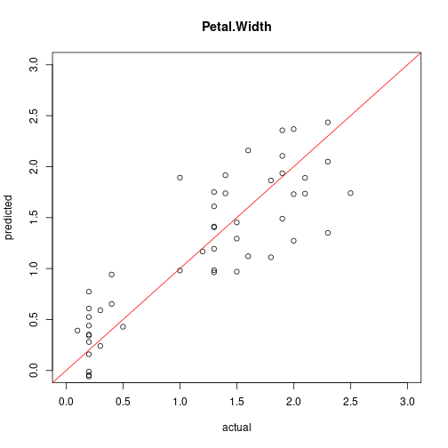
cor(test[,"Petal.Width"], predict(model4, test))
## [1] 0.8635826
Dummy coding is used for factors (i.e., levels are translated into individual 0-1 variable). The first level of factors is automatically used as the reference and the other levels are presented as 0-1 dummy variables called contrasts.
levels(train$Species)
## [1] "setosa" "versicolor" "virginica"
model.matrix is used internally to create the dummy coding.
head(model.matrix(Petal.Width ~ ., data=train))
##     (Intercept) Sepal.Length Sepal.Width Petal.Length  useless Speciesversicolor Speciesvirginica
## 85            1     2.980229    1.463570     5.227091 5.711515                 1                0
## 104           1     5.096036    3.043735     5.186573 6.568673                 0                1
## 30            1     4.361172    2.831668     1.860620 4.299253                 0                0
## 53            1     8.125130    2.405599     5.526070 6.123879                 1                0
## 143           1     6.371932    1.565055     6.147013 6.552573                 0                1
## 142           1     6.525973    3.696871     5.708392 5.221676                 0                1
Note that there is no dummy variable for species Setosa, because it is
used as the reference. It is often useful to set the reference level.
A simple way is to use the
function relevel to change which factor is listed first.
model6 <- step(lm(Petal.Width ~ ., data=train))
## Start:  AIC=-308.36
## Petal.Width ~ Sepal.Length + Sepal.Width + Petal.Length + useless +
##     Species
##
##                Df Sum of Sq     RSS     AIC
## - Sepal.Length  1    0.0062  3.9874 -310.20
## - Sepal.Width   1    0.0110  3.9921 -310.08
## - useless       1    0.0182  3.9994 -309.90
## <none>                       3.9812 -308.36
## - Petal.Length  1    0.4706  4.4518 -299.19
## - Species       2    8.7793 12.7605 -195.88
##
## Step:  AIC=-310.2
## Petal.Width ~ Sepal.Width + Petal.Length + useless + Species
##
##                Df Sum of Sq     RSS     AIC
## - Sepal.Width   1    0.0122  3.9996 -311.90
## - useless       1    0.0165  4.0039 -311.79
## <none>                       3.9874 -310.20
## - Petal.Length  1    0.4948  4.4822 -300.51
## - Species       2    8.8214 12.8087 -197.50
##
## Step:  AIC=-311.9
## Petal.Width ~ Petal.Length + useless + Species
##
##                Df Sum of Sq     RSS     AIC
## - useless       1    0.0185  4.0180 -313.44
## <none>                       3.9996 -311.90
## - Petal.Length  1    0.4836  4.4832 -302.48
## - Species       2    8.9467 12.9462 -198.44
##
## Step:  AIC=-313.44
## Petal.Width ~ Petal.Length + Species
##
##                Df Sum of Sq     RSS     AIC
## <none>                       4.0180 -313.44
## - Petal.Length  1    0.4977  4.5157 -303.76
## - Species       2    8.9310 12.9490 -200.41
model6
##
## Call:
## lm(formula = Petal.Width ~ Petal.Length + Species, data = train)
##
## Coefficients:
##       (Intercept)       Petal.Length  Speciesversicolor   Speciesvirginica
##           0.15970            0.06635            0.89382            1.49034
summary(model6)
##
## Call:
## lm(formula = Petal.Width ~ Petal.Length + Species, data = train)
##
## Residuals:
##      Min       1Q   Median       3Q      Max
## -0.72081 -0.14368  0.00053  0.12544  0.54598
##
## Coefficients:
##                   Estimate Std. Error t value Pr(>|t|)
## (Intercept)        0.15970    0.04413   3.619 0.000474 ***
## Petal.Length       0.06635    0.01924   3.448 0.000839 ***
## Speciesversicolor  0.89382    0.07459  11.984  < 2e-16 ***
## Speciesvirginica   1.49034    0.10203  14.607  < 2e-16 ***
## ---
## Signif. codes:  0 '***' 0.001 '**' 0.01 '*' 0.05 '.' 0.1 ' ' 1
##
## Residual standard error: 0.2046 on 96 degrees of freedom
## Multiple R-squared:  0.9302,	Adjusted R-squared:  0.928
## F-statistic: 426.5 on 3 and 96 DF,  p-value: < 2.2e-16
RMSE(predict(model6, test), test$Petal.Width)
## [1] 0.1885009
plot(test[,"Petal.Width"], predict(model6, test),
  xlim=c(0,3), ylim=c(0,3), xlab = "actual", ylab = "predicted",
  main = "Petal.Width")
abline(0,1, col="red")
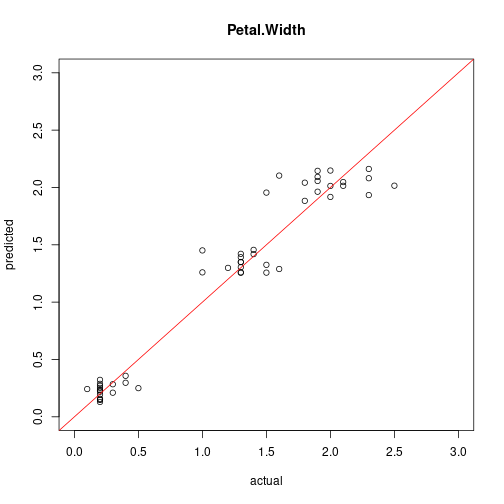
cor(test[,"Petal.Width"], predict(model6, test))
## [1] 0.9696326
Many models we use for classification can also perform regression to produce piece-wise predictors. For example CART:
library(rpart)
library(rpart.plot)
model7 <- rpart(Petal.Width ~ ., data=train,
  control=rpart.control(cp=0.01))
model7
## n= 100
##
## node), split, n, deviance, yval
##       * denotes terminal node
##
## 1) root 100 57.5739000 1.219000
##   2) Species=setosa 32  0.3796875 0.246875 *
##   3) Species=versicolor,virginica 68 12.7223500 1.676471
##     6) Species=versicolor 35  1.5354290 1.331429 *
##     7) Species=virginica 33  2.6006060 2.042424 *
rpart.plot(model7)
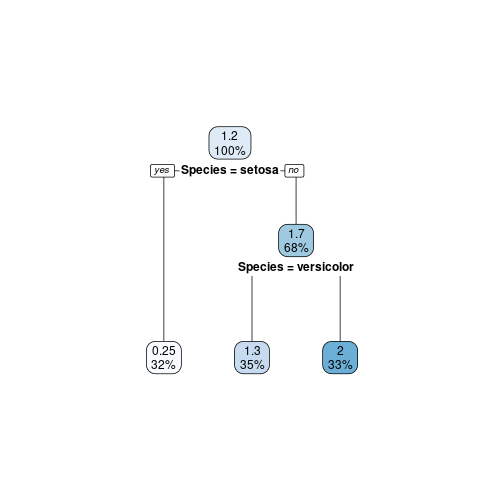
RMSE(predict(model7, test), test$Petal.Width)
## [1] 0.1819823
plot(test[,"Petal.Width"], predict(model7, test),
  xlim=c(0,3), ylim=c(0,3), xlab = "actual", ylab = "predicted",
  main = "Petal.Width")
abline(0,1, col="red")
cor(test[,"Petal.Width"], predict(model7, test))
## [1] 0.9716784
Note: This is not a nested model of the linear regressions so we cannot do ANOVA to compare the models!
LASSO and LAR try to reduce the number of parameters using a
regularization term (see lars in package lars and https://en.wikipedia.org/wiki/Elastic_net_regularization)
library(lars)
## Error in library(lars): there is no package called 'lars'
create a design matrix (with dummy variables and interaction terms).
lm did this automatically for us, but for this lars implementation
we have to do it manually.
x <- model.matrix(~ . + Sepal.Length*Sepal.Width*Petal.Length ,
  data = train[, -4])
head(x)
##     (Intercept) Sepal.Length Sepal.Width Petal.Length  useless Speciesversicolor Speciesvirginica
## 85            1     2.980229    1.463570     5.227091 5.711515                 1                0
## 104           1     5.096036    3.043735     5.186573 6.568673                 0                1
## 30            1     4.361172    2.831668     1.860620 4.299253                 0                0
## 53            1     8.125130    2.405599     5.526070 6.123879                 1                0
## 143           1     6.371932    1.565055     6.147013 6.552573                 0                1
## 142           1     6.525973    3.696871     5.708392 5.221676                 0                1
##     Sepal.Length:Sepal.Width Sepal.Length:Petal.Length Sepal.Width:Petal.Length
## 85                  4.361774                 15.577927                 7.650214
## 104                15.510984                 26.430965                15.786554
## 30                 12.349392                  8.114485                 5.268660
## 53                 19.545805                 44.900036                13.293508
## 143                 9.972422                 39.168344                 9.620411
## 142                24.125681                 37.252809                21.103190
##     Sepal.Length:Sepal.Width:Petal.Length
## 85                               22.79939
## 104                              80.44885
## 30                               22.97753
## 53                              108.01148
## 143                              61.30060
## 142                             137.71884
y <- train[, 4]

model_lars <- lars(x, y)
## Error in lars(x, y): could not find function "lars"
summary(model_lars)
## Error in eval(expr, envir, enclos): object 'model_lars' not found
model_lars
## Error in eval(expr, envir, enclos): object 'model_lars' not found
plot(model_lars)
## Error in eval(expr, envir, enclos): object 'model_lars' not found
the plot shows how variables are added (from left to right to the model)
find best model (using Mallows’s Cp statistic, see https://en.wikipedia.org/wiki/Mallows’s_Cp)
plot(model_lars, plottype = "Cp")
## Error in eval(expr, envir, enclos): object 'model_lars' not found
best <- which.min(model_lars$Cp)
## Error in eval(expr, envir, enclos): object 'model_lars' not found
coef(model_lars, s = best)
## Error in eval(expr, envir, enclos): object 'model_lars' not found
make predictions
x_test <- model.matrix(~ . + Sepal.Length*Sepal.Width*Petal.Length ,
  data = test[, -4])
predict(model_lars, x_test[1:5,], s = best)
## Error in eval(expr, envir, enclos): object 'model_lars' not found
test[1:5, ]$Petal.Width
## [1] 1.8 1.4 0.2 1.5 0.2
RMSE(predict(model_lars, x_test, s = best)$fit, test$Petal.Width)
## Error in eval(expr, envir, enclos): object 'model_lars' not found
plot(test[,"Petal.Width"],predict(model_lars, x_test, s = best)$fit,
  xlim=c(0,3), ylim=c(0,3), xlab = "actual", ylab = "predicted",
  main = "Petal.Width")
## Error in eval(expr, envir, enclos): object 'model_lars' not found
abline(0,1, col="red")
## Error in int_abline(a = a, b = b, h = h, v = v, untf = untf, ...): plot.new has not been called yet
cor(test[,"Petal.Width"], predict(model_lars, x_test, s = best)$fit)
## Error in eval(expr, envir, enclos): object 'model_lars' not found
roblm and robglm in package robustbase)glm)nlm)